Lane–Emden equation

Applications

Physically, hydrostatic equilibrium connects the gradient of the potential, the density, and the gradient of the pressure, whereas Poisson's equation connects the potential with the density. Thus, if we have a further equation that dictates how the pressure and density vary with respect to one another, we can reach a solution. The particular choice of a polytropic gas as given above makes the mathematical statement of the problem particularly succinct and leads to the Lane–Emden equation. The equation is a useful approximation for self-gravitating spheres of plasma such as stars, but typically it is a rather limiting assumption.

From hydrostatic equilibrium

Consider a self-gravitating, spherically symmetric fluid in hydrostatic equilibrium. Mass is conserved and thus described by the continuity equation

where ρ is a function of r . The equation of hydrostatic equilibrium is

where m is also a function of r . Differentiating again gives

where the continuity equation has been used to replace the mass gradient. Multiplying both sides by r 2 and collecting the derivatives of P on the left, one can write

Dividing both sides by r 2 yields, in some sense, a dimensional form of the desired equation. If, in addition, we substitute for the polytropic equation of state with P = K ρ c 1 + 1 n θ n + 1 and ρ = ρ c θ n , we have

Gathering the constants and substituting r = α ξ , where

we have the Lane–Emden equation,

From Poisson's equation

Equivalently, one can start with Poisson's equation,

One can replace the gradient of the potential using the hydrostatic equilibrium, via

which again yields the dimensional form of the Lane–Emden equation.

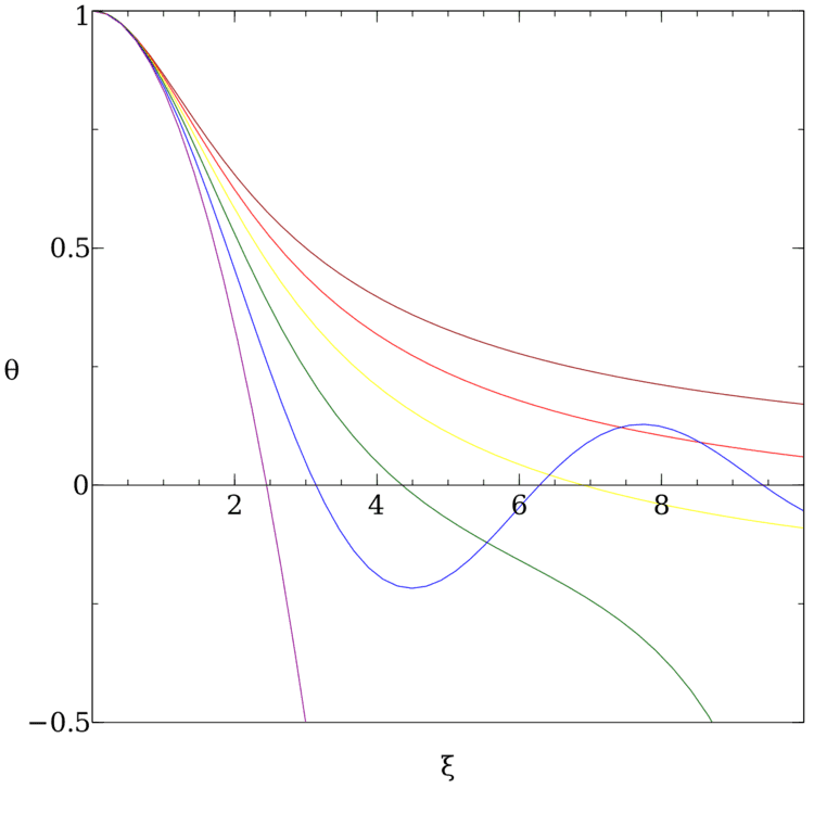
Solutions

For a given value of the polytropic index n , denote the solution to the Lane–Emden equation as θ n ( ξ ) . In general, the Lane–Emden equation must be solved numerically to find θ n . There are exact, analytic solutions for certain values of n , in particular: n = 0 , 1 , 5 . For n between 0 and 5, the solutions are continuous and finite in extent, with the radius of the star given by R = α ξ 1 , where θ n ( ξ 1 ) = 0 .

For a given solution θ n , the density profile is given by

The total mass M of the model star can be found by integrating the density over radius, from 0 to ξ 1 .

The pressure can be found using the polytropic equation of state, P = K ρ 1 + 1 n , i.e.

Finally, if the gas is ideal, the equation of state is P = k B ρ T / μ , where k B is the Boltzmann constant and μ the mean molecular weight. The temperature profile is then given by

Exact solutions

In spherically symmetric cases, the Lane-Emden equation is integrable for only three values of the polytropic index n .

For n = 0

If n = 0 , the equation becomes

Re-arranging and integrating once gives

Dividing both sides by ξ 2 and integrating again gives

The boundary conditions θ ( 0 ) = 1 and θ ′ ( 0 ) = 0 imply that the constants of integration are C 0 = 1 and C 1 = 0 .

For n = 1

When n = 1 , the equation can be expanded in the form

One assumes a power series solution:

This leads to a recursive relationship for the expansion coefficients:

This relation can be solved leading to the general solution:

The boundary condition for a physical polytrope demands that θ ( ξ ) → 1 as ξ → 0 . This requires that a 0 = 1 , a 1 = 0 , thus leading to the solution:

For n = 5

We start from with the Lane–Emden equation:

Rewriting for d θ 5 d ξ produces:

Differentiating with respect to ξ leads to:

Reduced, we come by:

Therefore, the Lane–Emden equation has the solution

when n = 5 . This solution is finite in mass but infinite in radial extent, and therefore the complete polytrope does not represent a physical solution.

Numerical solutions

In general, solutions are found by numerical integration. Many standard methods require that the problem is formulated as a system of first-order ordinary differential equations. For example,

Here, ϕ ( ξ ) is interpreted as the dimensionless mass, defined by m ( r ) = 4 π α 3 ρ c ϕ ( ξ ) . The relevant initial conditions are ϕ ( 0 ) = 0 and θ ( 0 ) = 1 . The first equation represents hydrostatic equilibrium and the second represents mass conservation.

Homology-invariant equation

It is known that if θ ( ξ ) is a solution of the Lane–Emden equation, then so is C 2 / n + 1 θ ( C ξ ) . Solutions that are related in this way are called homologous; the process that transforms them is homology. If one chooses variables that are invariant to homology, then we can reduce the order of the Lane–Emden equation by one.

A variety of such variables exist. A suitable choice is

and

We can differentiate the logarithms of these variables with respect to ξ , which gives

and

Finally, we can divide these two equations to eliminate the dependence on ξ , which leaves

This is now a single first-order equation.

Topology of the homology-invariant equation

The homology-invariant equation can be regarded as the autonomous pair of equations

and

The behaviour of solutions to these equations can be determined by linear stability analysis. The critical points of the equation (where d V / d log ⁡ ξ = d U / d log ⁡ ξ = 0 ) and the eigenvalues and eigenvectors of the Jacobian matrix are tabulated below.