Laguerre polynomials

The first few polynomials

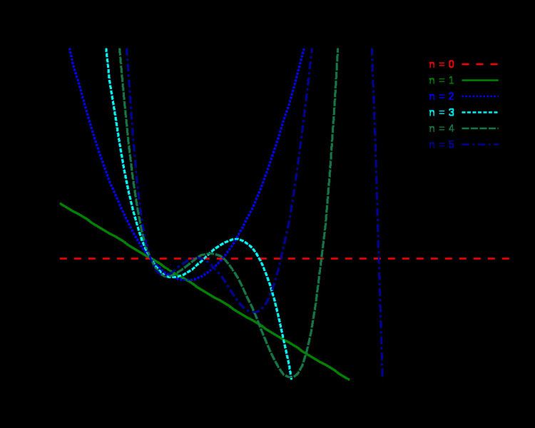
These are the first few Laguerre polynomials:

Recursive definition, closed form, and generating function

One can also define the Laguerre polynomials recursively, defining the first two polynomials as

L 0 ( x ) = 1 L 1 ( x ) = 1 − x

and then using the following recurrence relation for any k ≥ 1:

L k + 1 ( x ) = ( 2 k + 1 − x ) L k ( x ) − k L k − 1 ( x ) k + 1 .

The closed form is

L n ( x ) = ∑ k = 0 n ( n k ) ( − 1 ) k k ! x k .

The generating function for them likewise follows,

∑ n ∞ t n L n ( x ) = 1 1 − t e − t x 1 − t .

Polynomials of negative index can be expressed using the ones with positive index:

L − n ( x ) = e x L n − 1 ( − x ) .

Generalized Laguerre polynomials

For arbitrary real α the polynomial solutions of the differential equation

x y ″ + ( α + 1 − x ) y ′ + n y = 0

are called generalized Laguerre polynomials, or associated Laguerre polynomials.

One can also define the generalized Laguerre polynomials recursively, defining the first two polynomials as

L 0 ( α ) ( x ) = 1 L 1 ( α ) ( x ) = 1 + α − x

and then using the following recurrence relation for any k ≥ 1:

L k + 1 ( α ) ( x ) = ( 2 k + 1 + α − x ) L k ( α ) ( x ) − ( k + α ) L k − 1 ( α ) ( x ) k + 1 .

The simple Laguerre polynomials are the special case α = 0 of the generalized Laguerre polynomials:

L n ( 0 ) ( x ) = L n ( x ) .

The Rodrigues formula for them is

L n ( α ) ( x ) = x − α e x n ! d n d x n ( e − x x n + α ) = x − α ( d d x − 1 ) n n ! x n + α .

The generating function for them is

∑ n ∞ t n L n ( α ) ( x ) = 1 ( 1 − t ) α + 1 e − t x 1 − t .

Explicit examples and properties of the generalized Laguerre polynomials

Laguerre functions are defined by confluent hypergeometric functions and Kummer's transformation as

( n + α n ) is a generalized binomial coefficient. When n is an integer the function reduces to a polynomial of degree n. It has the alternative expression L n ( α ) ( x ) = ( − 1 ) n n ! U ( − n , α + 1 , x ) in terms of Kummer's function of the second kind.

The closed form for these generalized Laguerre polynomials of degree n is

derived by applying Leibniz's theorem for differentiation of a product to Rodrigues' formula.

The first few generalized Laguerre polynomials are:

The coefficient of the leading term is (−1)ⁿ/n!;

The constant term, which is the value at 0, is

If α is non-negative, then L_n^(α) has n real, strictly positive roots (notice that ( ( − 1 ) n − i L n − i ( α ) ) i = 0 n is a Sturm chain), which are all in the interval ( 0 , n + α + ( n − 1 ) n + α ] .

The polynomials' asymptotic behaviour for large n, but fixed α and x > 0, is given by

and summarizing by where J α is the Bessel function.

As a contour integral

Given the generating function specified above, the polynomials may be expressed in terms of a contour integral

L n ( α ) ( x ) = 1 2 π i ∮ C e − x t 1 − t ( 1 − t ) α + 1 t n + 1 d t ,

where the contour circles the origin once in a counterclockwise direction.

Recurrence relations

The addition formula for Laguerre polynomials:

L n ( α + β + 1 ) ( x + y ) = ∑ i = 0 n L i ( α ) ( x ) L n − i ( β ) ( y ) .

Laguerre's polynomials satisfy the recurrence relations

L n ( α ) ( x ) = ∑ i = 0 n L n − i ( α + i ) ( y ) ( y − x ) i i ! ,

in particular

L n ( α + 1 ) ( x ) = ∑ i = 0 n L i ( α ) ( x )

and

L n ( α ) ( x ) = ∑ i = 0 n ( α − β + n − i − 1 n − i ) L i ( β ) ( x ) ,

or

L n ( α ) ( x ) = ∑ i = 0 n ( α − β + n n − i ) L i ( β − i ) ( x ) ;

moreover

L n ( α ) ( x ) − ∑ j = 0 Δ − 1 ( n + α n − j ) ( − 1 ) j x j j ! = ( − 1 ) Δ x Δ ( Δ − 1 ) ! ∑ i = 0 n − Δ ( n + α n − Δ − i ) ( n − i ) ( n i ) L i ( α + Δ ) ( x ) = ( − 1 ) Δ x Δ ( Δ − 1 ) ! ∑ i = 0 n − Δ ( n + α − i − 1 n − Δ − i ) ( n − i ) ( n i ) L i ( n + α + Δ − i ) ( x )

They can be used to derive the four 3-point-rules

L n ( α ) ( x ) = L n ( α + 1 ) ( x ) − L n − 1 ( α + 1 ) ( x ) = ∑ j = 0 k ( k j ) L n − j ( α − k + j ) ( x ) , n L n ( α ) ( x ) = ( n + α ) L n − 1 ( α ) ( x ) − x L n − 1 ( α + 1 ) ( x ) , or  x k k ! L n ( α ) ( x ) = ∑ i = 0 k ( − 1 ) i ( n + i i ) ( n + α k − i ) L n + i ( α − k ) ( x ) , n L n ( α + 1 ) ( x ) = ( n − x ) L n − 1 ( α + 1 ) ( x ) + ( n + α ) L n − 1 ( α ) ( x ) x L n ( α + 1 ) ( x ) = ( n + α ) L n − 1 ( α ) ( x ) − ( n − x ) L n ( α ) ( x ) ;

combined they give this additional, useful recurrence relations

L n ( α ) ( x ) = ( 2 + α − 1 − x n ) L n − 1 ( α ) ( x ) − ( 1 + α − 1 n ) L n − 2 ( α ) ( x ) = α + 1 − x n L n − 1 ( α + 1 ) ( x ) − x n L n − 2 ( α + 2 ) ( x )

Since L n ( α ) ( x ) is a monic polynomial of degree n in α , there is the partial fraction decomposition

n ! L n ( α ) ( x ) ( α + 1 ) n = 1 − ∑ j = 1 n ( − 1 ) j j α + j ( n j ) L n ( − j ) ( x ) = 1 − ∑ j = 1 n x j α + j L n − j ( j ) ( x ) ( j − 1 ) ! = 1 − x ∑ i = 1 n L n − i ( − α ) ( x ) L i − 1 ( α + 1 ) ( − x ) α + i .

The second equality follows by the following identity, valid for integer i and n and immediate from the expression of L n ( α ) ( x ) in terms of Charlier polynomials:

( − x ) i i ! L n ( i − n ) ( x ) = ( − x ) n n ! L i ( n − i ) ( x ) .

For the third equality apply the fourth and fifth identities of this section.

Derivatives of generalized Laguerre polynomials

Differentiating the power series representation of a generalized Laguerre polynomial k times leads to

d k d x k L n ( α ) ( x ) = { ( − 1 ) k L n − k ( α + k ) ( x )  if  k ≤ n 0  otherwise .

This points to a special case (α = 0) of the formula above: for integer α = k the generalized polynomial may be written

L n ( k ) ( x ) = ( − 1 ) k d k L n + k ( x ) d x k ,

the shift by k sometimes causing confusion with the usual parenthesis notation for a derivative.

Moreover, the following equation holds:

1 k ! d k d x k x α L n ( α ) ( x ) = ( n + α k ) x α − k L n ( α − k ) ( x ) ,

which generalizes with Cauchy's formula to

L n ( α ′ ) ( x ) = ( α ′ − α ) ( α ′ + n α ′ − α ) ∫ 0 x t α ( x − t ) α ′ − α − 1 x α ′ L n ( α ) ( t ) d t .

The derivative with respect to the second variable α has the form,

d d α L n ( α ) ( x ) = ∑ i = 0 n − 1 L i ( α ) ( x ) n − i .

This is evident from the contour integral representation below.

The generalized Laguerre polynomials obey the differential equation

x L n ( α ) ′ ′ ( x ) + ( α + 1 − x ) L n ( α ) ′ ( x ) + n L n ( α ) ( x ) = 0 ,

which may be compared with the equation obeyed by the kth derivative of the ordinary Laguerre polynomial,

x L n [ k ] ′ ′ ( x ) + ( k + 1 − x ) L n [ k ] ′ ( x ) + ( n − k ) L n [ k ] ( x ) = 0 ,

where L n [ k ] ( x ) ≡ d k L n ( x ) d x k for this equation only.

In Sturm–Liouville form the differential equation is

− ( x α + 1 e − x ⋅ L n ( α ) ( x ) ′ ) ′ = n ⋅ x α e − x ⋅ L n ( α ) ( x ) ,

which shows that L(α)
n is an eigenvector for the eigenvalue n.

Orthogonality

The generalized Laguerre polynomials are orthogonal over [0, ∞) with respect to the measure with weighting function x^α e^−x:

∫ 0 ∞ x α e − x L n ( α ) ( x ) L m ( α ) ( x ) d x = Γ ( n + α + 1 ) n ! δ n , m ,

which follows from

∫ 0 ∞ x α ′ − 1 e − x L n ( α ) ( x ) d x = ( α − α ′ + n n ) Γ ( α ′ ) .

If Γ ( x , α + 1 , 1 ) denotes the Gamma distribution then the orthogonality relation can be written as

∫ 0 ∞ L n ( α ) ( x ) L m ( α ) ( x ) Γ ( x , α + 1 , 1 ) d x = ( n + α n ) δ n , m ,

The associated, symmetric kernel polynomial has the representations (Christoffel–Darboux formula)

K n ( α ) ( x , y ) := 1 Γ ( α + 1 ) ∑ i = 0 n L i ( α ) ( x ) L i ( α ) ( y ) ( α + i i ) = 1 Γ ( α + 1 ) L n ( α ) ( x ) L n + 1 ( α ) ( y ) − L n + 1 ( α ) ( x ) L n ( α ) ( y ) x − y n + 1 ( n + α n ) = 1 Γ ( α + 1 ) ∑ i = 0 n x i i ! L n − i ( α + i ) ( x ) L n − i ( α + i + 1 ) ( y ) ( α + n n ) ( n i ) ;

recursively

K n ( α ) ( x , y ) = y α + 1 K n − 1 ( α + 1 ) ( x , y ) + 1 Γ ( α + 1 ) L n ( α + 1 ) ( x ) L n ( α ) ( y ) ( α + n n ) .

Moreover,

y α e − y K n ( α ) ( ⋅ , y ) → δ ( y − ⋅ ) .

Turán's inequalities can be derived here, which is

L n ( α ) ( x ) 2 − L n − 1 ( α ) ( x ) L n + 1 ( α ) ( x ) = ∑ k = 0 n − 1 ( α + n − 1 n − k ) n ( n k ) L k ( α − 1 ) ( x ) 2 > 0.

The following integral is needed in the quantum mechanical treatment of the hydrogen atom,

∫ 0 ∞ x α + 1 e − x [ L n ( α ) ( x ) ] 2 d x = ( n + α ) ! n ! ( 2 n + α + 1 ) .

Series expansions

Let a function have the (formal) series expansion

f ( x ) = ∑ i = 0 ∞ f i ( α ) L i ( α ) ( x ) .

Then

f i ( α ) = ∫ 0 ∞ L i ( α ) ( x ) ( i + α i ) ⋅ x α e − x Γ ( α + 1 ) ⋅ f ( x ) d x .

The series converges in the associated Hilbert space L²[0, ∞) if and only if

∥ f ∥ L 2 2 := ∫ 0 ∞ x α e − x Γ ( α + 1 ) | f ( x ) | 2 d x = ∑ i = 0 ∞ ( i + α i ) | f i ( α ) | 2 < ∞ .

Further examples of expansions

Monomials are represented as

x n n ! = ∑ i = 0 n ( − 1 ) i ( n + α n − i ) L i ( α ) ( x ) ,

while binomials have the parametrization

( n + x n ) = ∑ i = 0 n α i i ! L n − i ( x + i ) ( α ) .

This leads directly to

e − γ x = ∑ i = 0 ∞ γ i ( 1 + γ ) i + α + 1 L i ( α ) ( x ) convergent iff  ℜ ( γ ) > − 1 2

for the exponential function. The incomplete gamma function has the representation

Γ ( α , x ) = x α e − x ∑ i = 0 ∞ L i ( α ) ( x ) 1 + i ( ℜ ( α ) > − 1 , x > 0 ) .

Multiplication theorems

Erdélyi gives the following two multiplication theorems

t n + 1 + α e ( 1 − t ) z L n ( α ) ( z t ) = ∑ k = n ( k n ) ( 1 − 1 t ) k − n L k ( α ) ( z ) , e ( 1 − t ) z L n ( α ) ( z t ) = ∑ k = 0 ( 1 − t ) k z k k ! L n ( α + k ) ( z ) .

Relation to Hermite polynomials

The generalized Laguerre polynomials are related to the Hermite polynomials:

H 2 n ( x ) = ( − 1 ) n 2 2 n n ! L n ( − 1 / 2 ) ( x 2 ) H 2 n + 1 ( x ) = ( − 1 ) n 2 2 n + 1 n ! x L n ( 1 / 2 ) ( x 2 )

where the H_n(x) are the Hermite polynomials based on the weighting function exp(−x²), the so-called "physicist's version."

Because of this, the generalized Laguerre polynomials arise in the treatment of the quantum harmonic oscillator.

Relation to hypergeometric functions

The Laguerre polynomials may be defined in terms of hypergeometric functions, specifically the confluent hypergeometric functions, as

L n ( α ) ( x ) = ( n + α n ) M ( − n , α + 1 , x ) = ( α + 1 ) n n ! 1 F 1 ( − n , α + 1 , x )

where ( a ) n is the Pochhammer symbol (which in this case represents the rising factorial).

Poisson kernel

∑ n = 0 ∞ n ! L n ( α ) ( x ) L n ( α ) ( y ) r n Γ ( 1 + α + n ) = exp ⁡ ( − ( x + y ) r 1 − r ) I α ( 2 x y r 1 − r ) ( x y r ) α 2 ( 1 − r ) , α > − 1 , | r | < 1.