Kramers–Kronig relations - Alchetron, the free social encyclopedia

Kramers kronig relations

The Kramers–Kronig relations are bidirectional mathematical relations, connecting the real and imaginary parts of any complex function that is analytic in the upper half-plane. These relations are often used to calculate the real part from the imaginary part (or vice versa) of response functions in physical systems, because for stable systems, causality implies the analyticity condition, and conversely, analyticity implies causality of the corresponding stable physical system. The relation is named in honor of Ralph Kronig and Hendrik Anthony Kramers. In mathematics these relations are known under the names Sokhotski–Plemelj theorem and Hilbert transform.

Formulation

Let χ ( ω ) = χ 1 ( ω ) + i χ 2 ( ω ) be a complex function of the complex variable ω , where χ 1 ( ω ) and χ 2 ( ω ) are real. Suppose this function is analytic in the closed upper half-plane of ω and vanishes like 1 / | ω | or faster as | ω | → ∞ . Slightly weaker conditions are also possible. The Kramers–Kronig relations are given by

χ 1 ( ω ) = 1 π P ∫ − ∞ ∞ χ 2 ( ω ′ ) ω ′ − ω d ω ′

and

χ 2 ( ω ) = − 1 π P ∫ − ∞ ∞ χ 1 ( ω ′ ) ω ′ − ω d ω ′ ,

where P denotes the Cauchy principal value. So the real and imaginary parts of such a function are not independent, and the full function can be reconstructed given just one of its parts.

Derivation

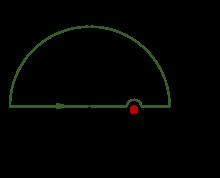
The proof begins with an application of Cauchy's residue theorem for complex integration. Given any analytic function χ in the closed upper half plane, the function ω ′ → χ ( ω ′ ) / ( ω ′ − ω ) where ω is real will also be analytic in the upper half of the plane. The residue theorem consequently states that

∮ χ ( ω ′ ) ω ′ − ω d ω ′ = 0

for any closed contour within this region. We choose the contour to trace the real axis, a hump over the pole at ω ′ = ω , and a large semicircle in the upper half plane. We then decompose the integral into its contributions along each of these three contour segments and pass them to limits. The length of the semicircular segment increases proportionally to | ω ′ | , but the integral over it vanishes in the limit because χ ( ω ′ ) vanishes at least as fast as 1 / | ω ′ | . We are left with the segments along the real axis and the half-circle around the pole. We pass the size of the half-circle to zero and obtain

0 = ∮ χ ( ω ′ ) ω ′ − ω d ω ′ = P ∫ − ∞ ∞ χ ( ω ′ ) ω ′ − ω d ω ′ − i π χ ( ω ) .

The second term in the last expression is obtained using the theory of residues, more specifically the Sokhotski–Plemelj theorem. Rearranging, we arrive at the compact form of the Kramers–Kronig relations,

χ ( ω ) = 1 i π P ∫ − ∞ ∞ χ ( ω ′ ) ω ′ − ω d ω ′ .

The single i in the denominator will effectuate the connection between the real and imaginary components. Finally, split χ ( ω ) and the equation into their real and imaginary parts to obtain the forms quoted above.

Physical interpretation and alternate form

We can apply the Kramers–Kronig formalism to response functions. In certain linear physical systems, or in engineering fields such as signal processing, the response function χ ( t − t ′ ) describes how some time-dependent property P ( t ) of a physical system responds to an impulse force F ( t ′ ) at time t ′ . For example, P ( t ) could be the angle of a pendulum and F ( t ) the applied force of a motor driving the pendulum motion. The response χ ( t − t ′ ) must be zero for t < t ′ since a system cannot respond to a force before it is applied. It can be shown (for instance, by invoking Titchmarsh's theorem) that this causality condition implies that the Fourier transform χ ( ω ) of χ ( t ) is analytic in the upper half plane. Additionally, if we subject the system to an oscillatory force with a frequency much higher than its highest resonant frequency, there will be almost no time for the system to respond before the forcing has switched direction, and so the frequency response χ ( ω ) will converge to zero as ω becomes very large. From these physical considerations, we see that χ ( ω ) will typically satisfy the conditions needed for the Kramers–Kronig relations to apply.

The imaginary part of a response function describes how a system dissipates energy, since it is out of phase with the driving force. The Kramers–Kronig relations imply that observing the dissipative response of a system is sufficient to determine its in-phase (reactive) response, and vice versa.

The integrals run from − ∞ to ∞ , implying we know the response at negative frequencies. Fortunately, in most systems, the positive frequency-response determines the negative-frequency response because χ ( ω ) is the Fourier transform of a real quantity χ ( t ) . We will make this assumption henceforth.

As a consequence, χ ( − ω ) = χ ∗ ( ω ) . This means χ 1 ( ω ) is an even function of frequency and χ 2 ( ω ) is odd.

Using these properties, we can collapse the integration ranges to [ 0 , ∞ ) . Consider the first relation, which gives the real part χ 1 ( ω ) . We transform the integral into one of definite parity by multiplying the numerator and denominator of the integrand by ω ′ + ω and separating:

χ 1 ( ω ) = 1 π P ∫ − ∞ ∞ ω ′ χ 2 ( ω ′ ) ω ′ 2 − ω 2 d ω ′ + ω π P ∫ − ∞ ∞ χ 2 ( ω ′ ) ω ′ 2 − ω 2 d ω ′ .

Since χ 2 ( ω ) is odd, the second integral vanishes, and we are left with

χ 1 ( ω ) = 2 π P ∫ 0 ∞ ω ′ χ 2 ( ω ′ ) ω ′ 2 − ω 2 d ω ′ .

The same derivation for the imaginary part gives

χ 2 ( ω ) = − 2 π P ∫ 0 ∞ ω χ 1 ( ω ′ ) ω ′ 2 − ω 2 d ω ′ = − 2 ω π P ∫ 0 ∞ χ 1 ( ω ′ ) ω ′ 2 − ω 2 d ω ′ .

These are the Kramers–Kronig relations in a form that is useful for physically realistic response functions.

Hu and Hall and Heck give a related and possibly more intuitive proof that avoids contour integration. It is based on the facts that:

A causal impulse response can be expressed as the sum of an even function and an odd function, where the odd function is the even function multiplied by the signum function.

The even and odd parts of a time domain waveform correspond to the real and imaginary parts of its Fourier integral, respectively.

Multiplication by the signum function in the time domain corresponds to the Hilbert transform (i.e. convolution by the Hilbert kernel) in the frequency domain.

Combining the formulas provided by these facts yields the Kramers–Kronig relations. This proof covers slightly different ground from the previous one in that it relates the real and imaginary parts in the frequency domain of any function that is causal in the time domain, offering an approach somewhat different from the condition of analyticity in the upper half plane of the frequency domain.

An article with an informal, pictorial version of this proof is also available.

Electron spectroscopy

In electron energy loss spectroscopy, Kramers–Kronig analysis allows one to calculate the energy dependence of both real and imaginary parts of a specimen's light optical permittivity, together with other optical properties such as the absorption coefficient and reflectivity.

In short, by measuring the number of high energy (e.g. 200 keV) electrons which lose a given amount of energy in traversing a very thin specimen (single scattering approximation), one can calculate the imaginary part of permittivity at that energy. Using this data with Kramers–Kronig analysis, one can calculate the real part of permittivity (as a function of energy) as well.

This measurement is made with electrons, rather than with light, and can be done with very high spatial resolution. One might thereby, for example, look for ultraviolet (UV) absorption bands in a laboratory specimen of interstellar dust less than a 100 nm across, i.e. too small for UV spectroscopy. Although electron spectroscopy has poorer energy resolution than light spectroscopy, data on properties in visible, ultraviolet and soft x-ray spectral ranges may be recorded in the same experiment.

In angle resolved photoemission spectroscopy the Kramers–Kronig relations can be used to link the real and imaginary parts of the electrons self energy. This is characteristic of the many body interaction the electron experiences in the material. Notable examples are in the high temperature superconductors, where kinks corresponding to the real part of the self energy are observed in the band dispersion and changes in the MDC width are also observed corresponding to the imaginary part of the self energy.

Hadronic scattering

The Kramers–Kronig relations are also used under the name "integral dispersion relations" with reference to hadronic scattering. In this case, the function is the scattering amplitude. Through the use of the optical theorem the imaginary part of the scattering amplitude is then related to the total cross section, which is a physically measurable quantity.

References

Kramers–Kronig relations Wikipedia

(Text) CC BY-SA