
 | ||
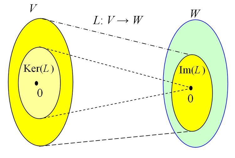
In mathematics, and more specifically in linear algebra and functional analysis, the kernel (also known as null space or nullspace) of a linear map L : V → W between two vector spaces V and W, is the set of all elements v of V for which L(v) = 0, where 0 denotes the zero vector in W. That is, in set-builder notation,
Contents
- Properties of the Kernel
- Application to modules
- The kernel in functional analysis
- Representation as matrix multiplication
- Subspace properties
- The row space of a matrix
- Left null space
- Nonhomogeneous systems of linear equations
- Illustration
- Examples
- Computation by Gaussian elimination
- Numerical computation
- Exact coefficients
- Floating point computation
- References
Properties of the Kernel
The kernel of L is a linear subspace of the domain V. In the linear map L : V → W, two elements of V have the same image in W if and only if their difference lies in the kernel of L:
It follows that the image of L is isomorphic to the quotient of V by the kernel:
This implies the rank–nullity theorem:
where, by “rank” we mean the dimension of the image of L, and by “nullity” that of the kernel of L.
When V is an inner product space, the quotient V / ker(L) can be identified with the orthogonal complement in V of ker(L). This is the generalization to linear operators of the row space, or coimage, of a matrix.
Application to modules
The notion of kernel applies to the homomorphisms of modules, the latter being a generalization of the vector space over a field to that over a ring. The domain of the mapping is a module, and the kernel constitutes a "submodule". Here, the concepts of rank and nullity do not necessarily apply.
The kernel in functional analysis
If V and W are topological vector spaces (and W is finite-dimensional) then a linear operator L: V → W is continuous if and only if the kernel of L is a closed subspace of V.
Representation as matrix multiplication
Consider a linear map represented as a m × n matrix A with coefficients in a field K (typically the field of the real numbers or of the complex numbers) and operating on column vectors x with n components over K. The kernel of this linear map is the set of solutions to the equation A x = 0, where 0 is understood as the zero vector. The dimension of the kernel of A is called the nullity of A. In set-builder notation,
The matrix equation is equivalent to a homogeneous system of linear equations:
Thus the kernel of A is the same as the solution set to the above homogeneous equations.
Subspace properties
The kernel of an m × n matrix A over a field K is a linear subspace of Kn. That is, the kernel of A, the set Null(A), has the following three properties:
- Null(A) always contains the zero vector, since A0 = 0.
- If x ∈ Null(A) and y ∈ Null(A), then x + y ∈ Null(A). This follows from the distributivity of matrix multiplication over addition.
- If x ∈ Null(A) and c is a scalar c ∈ K, then cx ∈ Null(A), since A(cx) = c(Ax) = c0 = 0.
The row space of a matrix
The product Ax can be written in terms of the dot product of vectors as follows:
Here a1, ... , am denote the transposed rows of the matrix A. It follows that x is in the kernel of A if and only if x is orthogonal (or perpendicular) to each of the row vectors of A (because when the dot product of two vectors is equal to zero, they are by definition orthogonal).
The row space, or coimage, of a matrix A is the span of the row vectors of A. By the above reasoning, the kernel of A is the orthogonal complement to the row space. That is, a vector x lies in the kernel of A if and only if it is perpendicular to every vector in the row space of A.
The dimension of the row space of A is called the rank of A, and the dimension of the kernel of A is called the nullity of A. These quantities are related by the rank–nullity theorem
Left null space
The left null space, or cokernel, of a matrix A consists of all vectors x such that xTA = 0T, where T denotes the transpose of a column vector. The left null space of A is the same as the kernel of AT. The left null space of A is the orthogonal complement to the column space of A, and is dual to the cokernel of the associated linear transformation. The kernel, the row space, the column space, and the left null space of A are the four fundamental subspaces associated to the matrix A.
Nonhomogeneous systems of linear equations
The kernel also plays a role in the solution to a nonhomogeneous system of linear equations:
If u and v are two possible solutions to the above equation, then
Thus, the difference of any two solutions to the equation Ax = b lies in the kernel of A.
It follows that any solution to the equation Ax = b can be expressed as the sum of a fixed solution v and an arbitrary element of the kernel. That is, the solution set to the equation Ax = b is
Geometrically, this says that the solution set to Ax = b is the translation of the kernel of A by the vector v. See also Fredholm alternative and flat (geometry).
Illustration
We give here a simple illustration of computing the kernel of a matrix (see the section Basis below for methods better suited to more complex calculations.) We also touch on the row space and its relation to the kernel.
Consider the matrix
The kernel of this matrix consists of all vectors (x, y, z) ∈ R3 for which
which can be expressed as a homogeneous system of linear equations involving x, y, and z:
which can be written in matrix form as:
Gauss–Jordan elimination reduces this to:
Rewriting yields:
Now we can express an element of the kernel:
for c a scalar.
Since c is a free variable, this can be expressed equally well as,
The kernel of A is precisely the solution set to these equations (in this case, a line through the origin in R3); the vector (−1,−26,16)T constitutes a basis of the kernel of A. Thus, the nullity of A is 1.
Note also that the following dot products are zero:
which illustrates that vectors in the kernel of A are orthogonal to each of the row vectors of A.
These two (linearly independent) row vectors span the row space of A, a plane orthogonal to the vector (−1,−26,16)T.
With the rank of A 2, the nullity of A 1, and the dimension of A 3, we have an illustration of the rank-nullity theorem.
Examples
Computation by Gaussian elimination
A basis of the kernel of a matrix may be computed by Gaussian elimination.
For this purpose, given an m × n matrix A, we construct first the row augmented matrix
Computing its column echelon form by Gaussian elimination (or any other suitable method), we get a matrix
In fact, the computation may be stopped as soon as the upper matrix is in column echelon form: the remainder of the computation consists in changing the basis of the vector space generated by the columns whose upper part is zero.
For example, suppose that
Then
Putting the upper part in column echelon form by column operations on the whole matrix gives
The last three columns of B are zero columns. Therefore, the three last vectors of C,
are a basis of the kernel of A.
Proof that the method computes the kernel: Since column operations correspond to post-multiplication by invertible matrices, the fact that
Numerical computation
The problem of computing the kernel on a computer depends on the nature of the coefficients.
Exact coefficients
If the coefficients of the matrix are exactly given numbers, the column echelon form of the matrix may be computed by Bareiss algorithm more efficiently than with Gaussian elimination. It is even more efficient to use modular arithmetic, which reduces the problem to a similar one over a finite field.
For coefficients in a finite field, Gaussian elimination works well, but for the large matrices that occur in cryptography and Gröbner basis computation, better algorithms are known, which have roughly the same computational complexity, but are faster and behave better with modern computer hardware.
Floating point computation
For matrices whose entries are floating-point numbers, the problem of computing the kernel makes sense only for matrices such that the number of rows is equal to their rank: because of the rounding errors, a floating-point matrix has almost always a full rank, even when it is an approximation of a matrix of a much smaller rank. Even for a full-rank matrix, it is possible to compute its kernel only if it is well conditioned, i.e. it has a low condition number.
Even for a well conditioned full rank matrix, Gaussian elimination does not behave correctly: it introduces rounding errors that are too large for getting a significant result. As the computation of the kernel of a matrix is a special instance of solving a homogeneous system of linear equations, the kernel may be computed by any of the various algorithms designed to solve homogeneous systems. A state of the art software for this purpose is the Lapack library.