Kepler's equation

Equation

Kepler's equation is

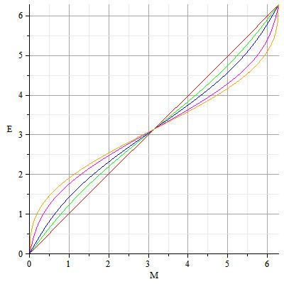
where M is the mean anomaly, E is the eccentric anomaly, and e is the eccentricity.

The 'eccentric anomaly' E is useful to compute the position of a point moving in a Keplerian orbit. As for instance, if the body passes the periastron at coordinates x = a(1 − e), y = 0, at time t = t₀, then to find out the position of the body at any time, you first calculate the mean anomaly M from the time and the mean motion n by the formula M = n(t − t₀), then solve the Kepler equation above to get E, then get the coordinates from:

Kepler's equation is a transcendental equation because sine is a transcendental function, meaning it cannot be solved for E algebraically. Numerical analysis and series expansions are generally required to evaluate E.

Alternate forms

There are several forms of Kepler's equation. Each form is associated with a specific type of orbit. The standard Kepler equation is used for elliptic orbits (0 ≤ e < 1). The hyperbolic Kepler equation is used for hyperbolic orbits (e ≫ 1). The radial Kepler equation is used for linear (radial) orbits (e = 1). Barker's equation is used for parabolic orbits (e = 1). When e = 1, Kepler's equation is not associated with an orbit.

When e = 0, the orbit is circular. Increasing e causes the circle to flatten into an ellipse. When e = 1, the orbit is completely flat, and it appears to be either a segment if the orbit is closed, or a ray if the orbit is open. An infinitesimal increase to e results in a hyperbolic orbit with a turning angle of 180 degrees, and the orbit appears to be a ray. Further increases reduce the turning angle, and as e goes to infinity, the orbit becomes a straight line of infinite length.

Hyperbolic Kepler equation

The Hyperbolic Kepler equation is:

where H is the hyperbolic eccentric anomaly. This equation is derived by multiplying Kepler's equation by the square root of −1; i = √−1 for imaginary unit, and replacing

to obtain

Radial Kepler equation

The Radial Kepler equation is:

where t is time, and x is the distance along an x-axis. This equation is derived by multiplying Kepler's equation by 1/2 making the replacement

and setting e = 1 gives

Inverse problem

Calculating M for a given value of E is straightforward. However, solving for E when M is given can be considerably more challenging.

Kepler's equation can be solved for E analytically by Lagrange inversion. The solution of Kepler's equation given by two Taylor series below.

Confusion over the solvability of Kepler's equation has persisted in the literature for four centuries. Kepler himself expressed doubt at the possibility of finding a general solution.

Inverse Kepler equation

The inverse Kepler equation is the solution of Kepler's equation for all real values of e :

Evaluating this yields:

These series can be reproduced in Mathematica with the InverseSeries operation.

These functions are simple Taylor series. Taylor series representations of transcendental functions are considered to be definitions of those functions. Therefore, this solution is a formal definition of the inverse Kepler equation. While this solution is the simplest in a certain mathematical sense, for values of e near 1 the convergence is very poor, other solutions are preferable for most applications. Alternatively, Kepler's equation can be solved numerically.

The solution for e ≠ 1 was discovered by Karl Stumpff in 1968, but its significance wasn't recognized.

Algorithm for the inverse Kepler equation

Note that E = m + e sin ⁡ E . Repeatedly substituting the expression on the right for the E on the right yields a simple fixed point iteration algorithm for evaluating E ( e , M ) .

The number of iterations, n , depends on the value of e .

Using Newton's method to find the zero of f = E − e sin ⁡ E − M one gets,

to first order in the small quantities M − E and e , or,

The algorithm actually uses a simplified version of Newton's method to improve on a value for E. Although Newton's method usually converges faster to the correct value for E there are situations where it requires division by 0 and the method above is then preferred.

Inverse radial Kepler equation

The inverse radial Kepler equation is:

Evaluating this yields:

To obtain this result using Mathematica:

Numerical approximation of inverse problem

For most applications, the inverse problem can be computed numerically by finding the root of the function:

This can be done iteratively via Newton's method:

Note that E and M are in units of radians in this computation. This iteration is repeated until desired accuracy is obtained (e.g. when f(E) < desired accuracy). For most elliptical orbits an initial value of E₀ = M(t) is sufficient. For orbits with e > 0.8, an initial value of E₀ = π should be used. A similar approach can be used for the hyperbolic form of Kepler's equation. In the case of a parabolic trajectory, Barker's equation is used.