
 | ||
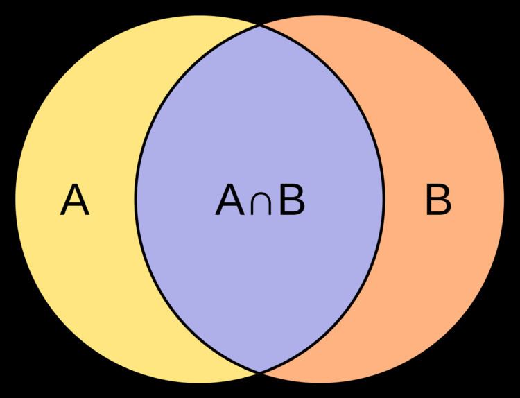
The Jaccard index, also known as the Jaccard similarity coefficient (originally coined coefficient de communauté by Paul Jaccard), is a statistic used for comparing the similarity and diversity of sample sets. The Jaccard coefficient measures similarity between finite sample sets, and is defined as the size of the intersection divided by the size of the union of the sample sets:
Contents
- Similarity of asymmetric binary attributes
- Difference with the simple matching coefficient SMC
- Generalized Jaccard similarity and distance
- Tanimoto similarity and distance
- Tanimotos definitions of similarity and distance
- Other definitions of Tanimoto distance
- References
(If A and B are both empty, we define J(A,B) = 1.)
The Jaccard distance, which measures dissimilarity between sample sets, is complementary to the Jaccard coefficient and is obtained by subtracting the Jaccard coefficient from 1, or, equivalently, by dividing the difference of the sizes of the union and the intersection of two sets by the size of the union:
An alternate interpretation of the Jaccard distance is as the ratio of the size of the symmetric difference
This distance is a metric on the collection of all finite sets.
There is also a version of the Jaccard distance for measures, including probability measures. If
The MinHash min-wise independent permutations locality sensitive hashing scheme may be used to efficiently compute an accurate estimate of the Jaccard similarity coefficient of pairs of sets, where each set is represented by a constant-sized signature derived from the minimum values of a hash function.
Similarity of asymmetric binary attributes
Given two objects, A and B, each with n binary attributes, the Jaccard coefficient is a useful measure of the overlap that A and B share with their attributes. Each attribute of A and B can either be 0 or 1. The total number of each combination of attributes for both A and B are specified as follows:
Each attribute must fall into one of these four categories, meaning that
The Jaccard similarity coefficient, J, is given as
The Jaccard distance, dJ, is given as
Difference with the simple matching coefficient (SMC)
When used for binary attributes, the Jaccard index is very similar to the simple matching coefficient. The main difference is that the SMC has the term
In market basket analysis, for example, the basket of two consumers who we wish to compare might only contain a small fraction of all the available products in the store, so the SMC will usually return very high values of similarities even when the baskets bear very little ressemblance, thus making the Jaccard index a more appropriate measure of similarity in that context. For example, consider a supermarket with 1000 products and two customers. The basket of the first customer contains salt and pepper and the basket of the second contains salt and sugar. In this scenario, the similarity between the two baskets as measured by the Jaccard index would be 1/3, but the similarity becomes 0.998 using the SMC.
In other contexts, where 0 and 1 carry equivalent information (symmetry), the SMC is a better measure of similarity. For example, vectors of demographic variables stored in dummies variables, such as gender, would be better compared with the SMC than with the Jaccard index since the impact of gender on similarity should be equal, independently of whether male is defined as a 0 and female as a 1 or the other way around. However, when we have symmetric dummy variables, one could replicate the behaviour of the SMC by splitting the dummies into two binary attributes (in this case, male and female), thus transforming them into asymmetric attributes, allowing the use of the Jaccard index without introducing any bias. By using this trick, the Jaccard index can be considered as making the SMC a fully redundant metric. The SMC remains, however, more computationally efficient in the case of symmetric dummy variables since it does not require adding extra dimensions.
Generalized Jaccard similarity and distance
If
and Jaccard distance
With even more generality, if
where
Then, for example, for two measurable sets
Tanimoto similarity and distance
Various forms of functions described as Tanimoto similarity and Tanimoto distance occur in the literature and on the Internet. Most of these are synonyms for Jaccard similarity and Jaccard distance, but some are mathematically different. Many sources cite an IBM Technical Report as the seminal reference. The report is available from several libraries.
In "A Computer Program for Classifying Plants", published in October 1960, a method of classification based on a similarity ratio, and a derived distance function, is given. It seems that this is the most authoritative source for the meaning of the terms "Tanimoto similarity" and "Tanimoto Distance". The similarity ratio is equivalent to Jaccard similarity, but the distance function is not the same as Jaccard distance.
Tanimoto's definitions of similarity and distance
In that paper, a "similarity ratio" is given over bitmaps, where each bit of a fixed-size array represents the presence or absence of a characteristic in the plant being modelled. The definition of the ratio is the number of common bits, divided by the number of bits set (i.e. nonzero) in either sample.
Presented in mathematical terms, if samples X and Y are bitmaps,
If each sample is modelled instead as a set of attributes, this value is equal to the Jaccard coefficient of the two sets. Jaccard is not cited in the paper, and it seems likely that the authors were not aware of it.
Tanimoto goes on to define a "distance coefficient" based on this ratio, defined for bitmaps with non-zero similarity:
This coefficient is, deliberately, not a distance metric. It is chosen to allow the possibility of two specimens, which are quite different from each other, to both be similar to a third. It is easy to construct an example which disproves the property of triangle inequality.
Other definitions of Tanimoto distance
Tanimoto distance is often referred to, erroneously, as a synonym for Jaccard distance
If Jaccard or Tanimoto similarity is expressed over a bit vector, then it can be written as
where the same calculation is expressed in terms of vector scalar product and magnitude. This representation relies on the fact that, for a bit vector (where the value of each dimension is either 0 or 1) then
This is a potentially confusing representation, because the function as expressed over vectors is more general, unless its domain is explicitly restricted. Properties of
There is a real danger that the combination of "Tanimoto Distance" being defined using this formula, along with the statement "Tanimoto Distance is a proper distance metric" will lead to the false conclusion that the function
Lipkus uses a definition of Tanimoto similarity which is equivalent to