Isoline retrieval

Rationale

Suppose we have, as in contour advection, inferred knowledge of a single contour or isoline of an atmospheric constituent, q and we wish to validate this against satellite remote-sensing data. Since satellite instruments cannot measure the constituent directly, we need to perform some sort of inversion. In order to validate the contour, it is not necessary to know, at any given point, the exact value of the constituent. We only need to know whether it falls inside or outside, that is, is it greater than or less than the value of the contour, q₀.

This is a classification problem. Let:

be the discretized variable. This will be related to the satellite measurement vector, y → , by some conditional probability, P ( y → | j ) , which we approximate by collecting samples, called training data, of both the measurement vector and the state variable, q. By generating classification results over the region of interest and using any contouring algorithm to separate the two classes, the isoline will have been "retrieved."

The accuracy of a retrieval will be given by integrating the conditional probability over the area of interest, A:

where c is the retrieved class at position, r → . We can maximize this quantity by maximizing the value of the integrand at each point:

Since this is the definition of maximum likelihood, a classification algorithm based on maximum likelihood is the most accurate method possible of validating an advected contour. A good method for performing maximum likelihood classification from a set of training data is variable kernel density estimation.

Training data

There are two methods of generating the training data. The most obvious is empirically, by simply matching measurements of the variable, q, with collocated measurements from the satellite instrument. In this case, no knowledge of the actual physics that produce the measurement is required and the retrieval algorithm is purely statistical. The second is with a forward model:

where x → is the state vector and q = x_k is a single component. An advantage of this method is that state vectors need not reflect actual atmospheric configurations, they need only take on a state that could reasonably occur in the real atmosphere. There are also none of the errors inherent in most collocation procedures, e.g. because of offset errors in the locations of the paired samples and differences in the footprint sizes of the two instruments. Since retrievals will be biased towards more common states, however, the statistics ought to reflect those in the real world.

Error characterization

The conditional probabilities, P ( y → | j ) , provide excellent error characterization, therefore the classification algorithm ought to return them. We define the confidence rating by rescaling the conditional probability:

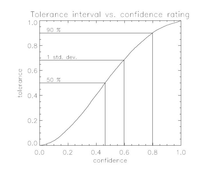
where n_c is the number of classes (in this case, two). If C is zero, then the classification is little better than chance, while if it is one, then it should be perfect. To transform the confidence rating to a statistical tolerance, the following line integral can be applied to an isoline retrieval for which the true isoline is known:

where s is the path, l is the length of the isoline and C ′ is the retrieved confidence as a function of position. While it appears that the integral must be evaluated separately for each value of the confidence rating, C, in fact it may be done for all values of C by sorting the confidence ratings of the results, C ′ . The function relates the threshold value of the confidence rating for which the tolerance is applicable. That is, it defines a region that contains a fraction of the true isoline equal to the tolerance.

Example: water vapour from AMSU

The Advanced Microwave Sounding Unit (AMSU) series of satellite instruments are designed to detect temperature and water vapour. They have a high horizontal resolution (as little as 15 km) and because they are mounted on more than one satellite, full global coverage can be obtained in less than one day. Training data was generated using the second method from European Centre for Medium-Range Weather Forecasts (ECMWF) ERA-40 data fed to a fast radiative transfer model called RTTOV. The function, δ ( C ) has been generated from simulated retrievals and is shown in the figure to the right. This is then used to set the 90 percent tolerance in the figure below by shading all the confidence ratings less than 0.8. Thus we expect the true isoline to fall within the shading 90 percent of the time.

For continuum retrievals

Isoline retrieval is also useful for retrieving a continuum variable and constitutes a general, nonlinear inverse method. It has the advantage over both a neural network, as well as iterative methods such as optimal estimation that invert the forward model directly, in that there is no possibility of getting stuck in a local minimum.

There are a number of methods of reconstituting the continuum variable from the discretized one. Once a sufficient number of contours have been retrieved, it is straightforward to interpolate between them. Conditional probabilities make a good proxy for the continuum value.

Consider the transformation from a continuum to a discrete variable:

Suppose that P ( q | y → ) is given by a Gaussian:

where q ¯ is the expectation value and σ q is the standard deviation, then the conditional probability is related to the continuum variable, q, by the error function:

The figure shows conditional probability versus specific humidity for the example retrieval discussed above.

As a robust estimator

The location of q₀ is found by setting the conditional probabilities of the two classes to be equal:

In other words, equal amounts of the "zeroeth order moment" lie on either side of q₀. This type of formulation is characteristic of a robust estimator.