
Parameters n ∈ N0 | ||
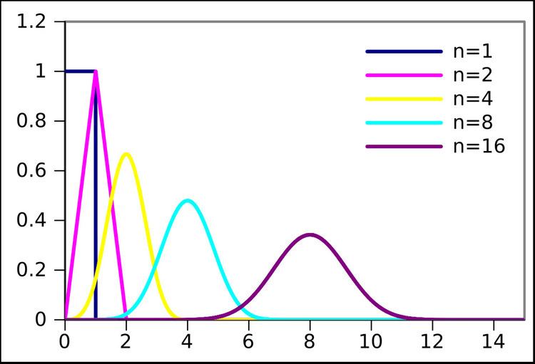 | ||
Support x ∈ [ 0 , n ] {\displaystyle x\in [0,n]} PDF 1 ( n − 1 ) ! ∑ k = 0 ⌊ x ⌋ ( − 1 ) k ( n k ) ( x − k ) n − 1 {\displaystyle {\frac {1}{(n-1)!}}\sum _{k=0}^{\lfloor x\rfloor }(-1)^{k}{\binom {n}{k}}(x-k)^{n-1}} CDF 1 n ! ∑ k = 0 ⌊ x ⌋ ( − 1 ) k ( n k ) ( x − k ) n {\displaystyle {\frac {1}{n!}}\sum _{k=0}^{\lfloor x\rfloor }(-1)^{k}{\binom {n}{k}}(x-k)^{n}} Mean n 2 {\displaystyle {\frac {n}{2}}} Median n 2 {\displaystyle {\frac {n}{2}}} | ||
In probability and statistics, the Irwin–Hall distribution, named after Joseph Oscar Irwin and Philip Hall, is a probability distribution for a random variable defined as the sum of a number of independent random variables, each having a uniform distribution. For this reason it is also known as the uniform sum distribution.
Contents
- Definition
- Special cases
- Similar and related distributions
- Extensions to the Irwin Hall Distribution
- References
The generation of pseudo-random numbers having an approximately normal distribution is sometimes accomplished by computing the sum of a number of pseudo-random numbers having a uniform distribution; usually for the sake of simplicity of programming. Rescaling the Irwin–Hall distribution provides the exact distribution of the random variates being generated.
This distribution is sometimes confused with the Bates distribution, which is the mean (not sum) of n independent random variables uniformly distributed from 0 to 1.
Definition
The Irwin–Hall distribution is the continuous probability distribution for the sum of n independent and identically distributed U(0, 1) random variables:
The probability density function (pdf) is given by
where sgn(x − k) denotes the sign function:
Thus the pdf is a spline (piecewise polynomial function) of degree n − 1 over the knots 0, 1, ..., n. In fact, for x between the knots located at k and k + 1, the pdf is equal to
where the coefficients aj(k,n) may be found from a recurrence relation over k
The coefficients are also A188816 in OEIS. The coefficients for the cumulative distribution is A188668.
The mean and variance are n/2 and n/12, respectively.
Special cases
Similar and related distributions
The Irwin-Hall distribution is similar to the Bates distribution, but still featuring only integers as parameter. An extension to real-valued parameters is possible by adding also a random uniform variable with N-trunc(N) as width.
Extensions to the Irwin-Hall Distribution
When using the Irwin-Hall for data fitting purposes one problem is that the IH is not very flexible because the parameter n needs to be an integer. However, instead of summing n equal uniform distributions, we could also add e.g. U+0.5U to address also the case n=1.5 (giving a trapezoidal distribution).