In mathematics, the inverse of a function
y
=
f
(
x
)
is a function that, in some fashion, "undoes" the effect of
f
(see inverse function for a formal and detailed definition). The inverse of
f
is denoted
f
−
1
. The statements y = f(x) and x = f −1(y) are equivalent.
Their two derivatives, assuming they exist, are reciprocal, as the Leibniz notation suggests; that is:
d
x
d
y
⋅
d
y
d
x
=
1.
This is a direct consequence of the chain rule, since
d
x
d
y
⋅
d
y
d
x
=
d
x
d
x
and the derivative of
x
with respect to
x
is 1.
Writing explicitly the dependence of
y
on
x
and the point at which the differentiation takes place and using Lagrange's notation, the formula for the derivative of the inverse becomes
[
f
−
1
]
′
(
a
)
=
1
f
′
(
f
−
1
(
a
)
)
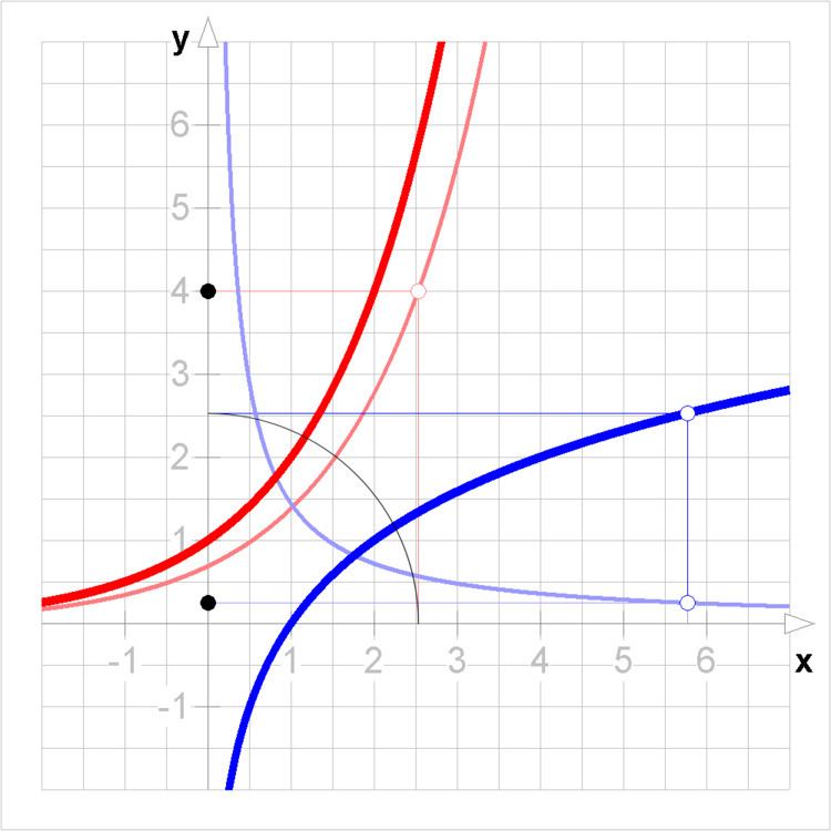
Geometrically, a function and inverse function have graphs that are reflections, in the line y = x. This reflection operation turns the gradient of any line into its reciprocal.
Assuming that
f
has an inverse in a neighbourhood of
x
and that its derivative at that point is non-zero, its inverse is guaranteed to be differentiable at
x
and have a derivative given by the above formula.
y
=
x
2
(for positive
x
) has inverse
x
=
y
.
d
y
d
x
=
2
x
;
d
x
d
y
=
1
2
y
=
1
2
x
d
y
d
x
⋅
d
x
d
y
=
2
x
⋅
1
2
x
=
1.
At x = 0, however, there is a problem: the graph of the square root function becomes vertical, corresponding to a horizontal tangent for the square function.
y
=
e
x
(for real
x
) has inverse
x
=
ln
y
(for positive
y
)
d
y
d
x
=
e
x
;
d
x
d
y
=
1
y
d
y
d
x
⋅
d
x
d
y
=
e
x
⋅
1
y
=
e
x
e
x
=
1
Integrating this relationship gives
This is only useful if the integral exists. In particular we need
f
′
(
x
)
to be non-zero across the range of integration.
It follows that a function that has a continuous derivative has an inverse in a neighbourhood of every point where the derivative is non-zero. This need not be true if the derivative is not continuous.
The chain rule given above is obtained by differentiating the identity x = f −1(f(x)) with respect to x. One can continue the same process for higher derivatives. Differentiating the identity twice with respect to x , one obtains
d
2
y
d
x
2
⋅
d
x
d
y
+
d
d
x
(
d
x
d
y
)
⋅
(
d
y
d
x
)
=
0
,
that is simplified further by the chain rule as
d
2
y
d
x
2
⋅
d
x
d
y
+
d
2
x
d
y
2
⋅
(
d
y
d
x
)
2
=
0.
Replacing the first derivative, using the identity obtained earlier, we get
d
2
y
d
x
2
=
−
d
2
x
d
y
2
⋅
(
d
y
d
x
)
3
.
Similarly for the third derivative:
d
3
y
d
x
3
=
−
d
3
x
d
y
3
⋅
(
d
y
d
x
)
4
−
3
d
2
x
d
y
2
⋅
d
2
y
d
x
2
⋅
(
d
y
d
x
)
2
or using the formula for the second derivative,
d
3
y
d
x
3
=
−
d
3
x
d
y
3
⋅
(
d
y
d
x
)
4
+
3
(
d
2
x
d
y
2
)
2
⋅
(
d
y
d
x
)
5
These formulas are generalized by the Faà di Bruno's formula.
These formulas can also be written using Lagrange's notation. If f and g are inverses, then
g
″
(
x
)
=
−
f
″
(
g
(
x
)
)
[
f
′
(
g
(
x
)
)
]
3
y
=
e
x
has the inverse
x
=
ln
y
. Using the formula for the second derivative of the inverse function,
d
y
d
x
=
d
2
y
d
x
2
=
e
x
=
y
;
(
d
y
d
x
)
3
=
y
3
;
so that
d
2
x
d
y
2
⋅
y
3
+
y
=
0
;
d
2
x
d
y
2
=
−
1
y
2
,
which agrees with the direct calculation.