
 | ||
In algebraic geometry, a hyperelliptic curve is an algebraic curve given by an equation of the form
Contents
- Genus of the curve
- Formulation and choice of model
- Using Riemann Hurwitz formula
- Occurrence and applications
- Classification
- Example
- History
- References
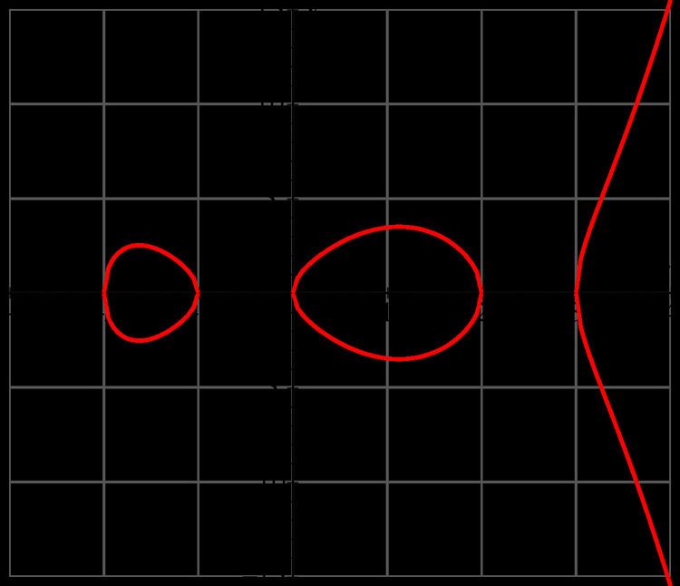
where f(x) is a polynomial of degree n > 4 with n distinct roots. A hyperelliptic function is an element of the function field of such a curve or possibly of the Jacobian variety on the curve, these two concepts being the same in the elliptic function case, but different in the present case. Fig. 1 is the graph of
Genus of the curve
The degree of the polynomial determines the genus of the curve: a polynomial of degree 2g + 1 or 2g + 2 gives a curve of genus g. When the degree is equal to 2g + 1, the curve is called an imaginary hyperelliptic curve. Meanwhile, a curve of degree 2g + 2 is termed a real hyperelliptic curve. This statement about genus remains true for g = 0 or 1, but those curves are not called "hyperelliptic". Rather, the case g = 1 (if we choose a distinguished point) is an elliptic curve. Hence the terminology.
Formulation and choice of model
While this model is the simplest way to describe hyperelliptic curves, such an equation will have a singular point at infinity in the projective plane. This feature is specific to the case n > 4. Therefore, in giving such an equation to specify a non-singular curve, it is almost always assumed that a non-singular model (also called a smooth completion), equivalent in the sense of birational geometry, is meant.
To be more precise, the equation defines a quadratic extension of C(x), and it is that function field that is meant. The singular point at infinity can be removed (since this is a curve) by the normalization (integral closure) process. It turns out that after doing this, there is an open cover of the curve by two affine charts: the one already given by
and another one given by
The glueing maps between the two charts are given by
and
wherever they are defined.
In fact geometric shorthand is assumed, with the curve C being defined as a ramified double cover of the projective line, the ramification occurring at the roots of f, and also for odd n at the point at infinity. In this way the cases n = 2g + 1 and 2g + 2 can be unified, since we might as well use an automorphism of the projective line to move any ramification point away from infinity.
Using Riemann-Hurwitz formula
Using Riemann-Hurwitz formula, the hyperelliptic curve with genus g is defined by an equation with degree n = 2g + 2. Suppose the bijective morphism f : X → P1 with ramification degree 2, where X is a curve with genus g and P1 is the Riemann sphere. Let g1 = g and g0 be the genus of P1 ( = 0 ), then the Riemann-Hurwitz formula turns out to be
where s is over all ramified points on X. The number of ramified points is finite, n, so n = 2g + 2.
Occurrence and applications
All curves of genus 2 are hyperelliptic, but for genus ≥ 3 the generic curve is not hyperelliptic. This is seen heuristically by a moduli space dimension check. Counting constants, with n = 2g + 2, the collection of n points subject to the action of the automorphisms of the projective line has (2g + 2) − 3 degrees of freedom, which is less than 3g − 3, the number of moduli of a curve of genus g, unless g is 2. Much more is known about the hyperelliptic locus in the moduli space of curves or abelian varieties, though it is harder to exhibit general non-hyperelliptic curves with simple models. One geometric characterization of hyperelliptic curves is via Weierstrass points. More detailed geometry of non-hyperelliptic curves is read from the theory of canonical curves, the canonical mapping being 2-to-1 on hyperelliptic curves but 1-to-1 otherwise for g > 2. Trigonal curves are those that correspond to taking a cube root, rather than a square root, of a polynomial.
The definition by quadratic extensions of the rational function field works for fields in general except in characteristic 2; in all cases the geometric definition as a ramified double cover of the projective line is available, if it is assumed to be separable.
Hyperelliptic curves can be used in hyperelliptic curve cryptography for cryptosystems based on the discrete logarithm problem.
Hyperelliptic curves also appear composing entire connected components of certain strata of the moduli space of Abelian differentials.
Classification
Hyperelliptic curves of given genus g have a moduli space, closely related to the ring of invariants of a binary form of degree 2g+2.
Example
See Bolza surface
History
Hyperelliptic functions were first published by Adolph Göpel (1812-1847) in his last paper Abelsche Transcendenten erster Ordnung (Abelian transcendents of first order) (in Journal für reine und angewandte Mathematik, vol. 35, 1847). Independently Johann G. Rosenhain worked on that matter and published Umkehrungen ultraelliptischer Integrale erster Gattung (in Mémoires des sa vanta etc., vol. 11, 1851).