Hyperbolic discounting - Alchetron, The Free Social Encyclopedia

In economics, hyperbolic discounting is a time-inconsistent model of discounting.

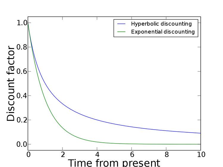
Given two similar rewards, humans show a preference for one that arrives sooner rather than later. Humans are said to discount the value of the later reward, by a factor that increases with the length of the delay. This process is traditionally modeled in the form of exponential discounting, a time-consistent model of discounting. A large number of studies have since demonstrated that the constant discount rate assumed in exponential discounting is systematically being violated. Hyperbolic discounting is a particular mathematical model devised as an alternative to exponential discounting.

According to hyperbolic discounting, valuations fall relatively rapidly for earlier delay periods (as in, from now to one week), but then fall more slowly for longer delay periods (from ten weeks to 21). This contrasts with exponential discounting, in which valuation falls by a constant factor per unit delay. The standard experiment used to reveal a test subject's hyperbolic discounting curve is to compare short-term preferences with long-term preferences. For instance: "Would you prefer a dollar today or three dollars tomorrow?" or "Would you prefer a dollar in one year or three dollars in one year and one day?" It has been claimed that a significant fraction of subjects will take the lesser amount today, but will gladly wait one extra day in a year in order to receive the higher amount instead. Individuals with such preferences are described as "present-biased".

Individuals using hyperbolic discounting reveal a strong tendency to make choices that are inconsistent over time – they make choices today that their future self would prefer not to have made, despite using the same reasoning. This dynamic inconsistency happens because the value of future rewards is much lower under hyperbolic discounting than under exponential discounting.

Observations

The phenomenon of hyperbolic discounting is implicit in Richard Herrnstein's "matching law", which states that when dividing their time or effort between two non-exclusive, ongoing sources of reward, most subjects allocate in direct proportion to the rate and size of rewards from the two sources, and in inverse proportion to their delays. That is, subjects' choices "match" these parameters.

After the report of this effect in the case of delay, George Ainslie pointed out that in a single choice between a larger, later and a smaller, sooner reward, inverse proportionality to delay would be described by a plot of value by delay that had a hyperbolic shape, and that when the larger, later reward is preferred, this preference can be reversed by reducing both rewards' delays by the same absolute amount. That is, for values of x for which under current conditions it would be obviously rational to prefer x dollars in (n + 1) days over one dollar in n days (e.g., x = 3), a large subset of the population would (rationally) prefer the former alternative given large values of n, but even among this subset, a large (sub-)subset would (irrationally) prefer one dollar in n days when n = 0. Ainslie demonstrated the predicted reversal to occur among pigeons.

A large number of subsequent experiments have confirmed that spontaneous preferences by both human and nonhuman subjects follow a hyperbolic curve rather than the conventional, "exponential" curve that would produce consistent choice over time. For instance, when offered the choice between $50 now and $100 a year from now, many people will choose the immediate $50. However, given the choice between $50 in five years or $100 in six years almost everyone will choose $100 in six years, even though that is the same choice seen at five years' greater distance.

Hyperbolic discounting has also been found to relate to real-world examples of self-control. Indeed, a variety of studies have used measures of hyperbolic discounting to find that drug-dependent individuals discount delayed consequences more than matched nondependent controls, suggesting that extreme delay discounting is a fundamental behavioral process in drug dependence. Some evidence suggests pathological gamblers also discount delayed outcomes at higher rates than matched controls. Whether high rates of hyperbolic discounting precede addictions or vice versa is currently unknown, although some studies have reported that high-rate discounters are more likely to consume alcohol and cocaine than lower-rate discounters. Likewise, some have suggested that high-rate hyperbolic discounting makes unpredictable (gambling) outcomes more satisfying.

The degree of discounting is vitally important in describing hyperbolic discounting, especially in the discounting of specific rewards such as money. The discounting of monetary rewards varies across age groups due to the varying discount rate. The rate depends on a variety of factors, including the species being observed, age, experience, and the amount of time needed to consume the reward.

Criticism

An article from 2003 noted that the evidence might be better explained by a similarity heuristic than by hyperbolic discounting. Similarly, a 2011 paper criticized the existing studies for mostly using data collected from university students and being too quick to conclude that the hyperbolic model of discounting is correct.

A study by Daniel Read introduces "subadditive discounting": the fact that discounting over a delay increases if the delay is divided into smaller intervals. This hypothesis may explain the main finding of many studies in support of hyperbolic discounting—the observation that impatience declines with time–while also accounting for observations not predicted by hyperbolic discounting.

Step-by-step explanation

Suppose that in a study, participants are offered the choice between taking x dollars immediately or taking y dollars n days later. Suppose further that one participant in that study employs exponential discounting and another employs hyperbolic discounting.

Each participant will realize that a) they should take x dollars immediately if they can invest the dollar in a different venture that will yield more than y dollars n days later and b) they will be indifferent between the choices (selecting one at random) if the best available alternative will likewise yield y dollars n days later. (Assume, for the sake of simplicity, that the values of all available investments are compounded daily.) Each participant correctly understands the fundamental question being asked: "For any given value of y dollars and n days, what is the minimum amount of money, i.e., the minimum value for x dollars, that I should be willing to accept? In other words, how many dollars would I need to invest today to get y dollars n days from now?" Each will take x dollars if x is greater than the answer that they calculate, and each will take y dollars n days from now if x is smaller than that answer. However, the methods that they use to calculate that amount and the answers that they get will be different, and only the exponential discounter will use the correct method and get a reliably correct result:

The exponential discounter will think "The best alternative investment available (that is, the best investment available in the absence of this choice) gives me a return of r percent per day; in other words, once a day it adds to its value r percent of the value that it had the previous day. That is, every day it multiplies its value once by (100% + r%). So if I hold the investment for n days, its value will have multiplied itself by this amount n times, making that value (100% + r%)^n of what it was at the start – that is, (1 + r%)^n times what it was at the start. So to figure out how much I would need to start with today to get y dollars n days from now, I need to divide y dollars by ([1 + r%]^n). If my other choice of how much money to take is greater than this result, then I should take the other amount, invest it in the other venture that I have in mind, and get even more at the end. If this result is greater than my other choice, then I should take y dollars n days from now, because it turns out that by giving up the other choice I am essentially investing that smaller amount of money to get y dollars n days from now, meaning that I'm getting an even greater return by waiting n days for y dollars, making this my best available investment."

The hyperbolic discounter, however, will think "If I want y dollars n days from now, then the amount that I need to invest today is y divided by n, because that amount times n equals y dollars. [There lies the hyperbolic discounter's error.] If my other choice is greater than this result, I should take it instead because x times n will be greater than y times n; if it is less than this result, then I should wait n days for y dollars."

Where the exponential discounter reasons correctly and the hyperbolic discounter goes wrong is that as n becomes very large, the value of ([1 + r%]^n) becomes much larger than the value of n, with the effect that the value of (y/[(1 + r%)^n) becomes much smaller than the value of (y/n). Therefore, the minimum value of x (the number of dollars in the immediate choice) that suffices to be greater than that amount will be much smaller than the hyperbolic discounter thinks, with the result that they will perceive x-values in the range from (y/[(1 + r%)^n) to (y/n) (inclusive at the low end) as being too small and, as a result, irrationally turn those alternatives down when they are in fact the better investment.

Formal model

Hyperbolic discounting is mathematically described as:

f H ( D ) = 1 1 + k D

where f(D) is the discount factor that multiplies the value of the reward, D is the delay in the reward, and k is a parameter governing the degree of discounting. This is compared with the formula for exponential discounting:

f E ( D ) = e − k D

Simple derivation

If f ( n ) = 2 − n is an exponential discounting function and g ( n ) = 1 1 + n a hyperbolic function (with n the amount of weeks), then the exponential discounting a week later from "now" (n=0) is f ( 1 ) f ( 0 ) = 1 2 , and the exponential discounting a week from week n is f ( n + 1 ) f ( n ) = 1 2 , which means they are the same. For g(n), g ( 1 ) g ( 0 ) = 1 2 , which is the same as for f, while g ( n + 1 ) g ( n ) = 1 − 1 n + 2 . From this one can see that the two types of discounting are the same "now", but when n is much greater than 1, for instance 52 (one year), g ( n + 1 ) g ( n ) will tend to go to 1, so that the hyperbolic discounting of a week in the far future is virtually zero, while the exponential is still 1/2.

Quasi-hyperbolic approximation

The "quasi-hyperbolic" discount function, proposed by Laibson (1997), approximates the hyperbolic discount function above in discrete time by

f Q H ( 0 ) = 1 ,

and

f Q H ( D ) = β × δ D ,

where β and δ are constants between 0 and 1; and again D is the delay in the reward, and f(D) is the discount factor. The condition f(0) = 1 is stating that rewards taken at the present time are not discounted.

Quasi-hyperbolic time preferences are also referred to as "beta-delta" preferences. They retain much of the analytical tractability of exponential discounting while capturing the key qualitative feature of discounting with true hyperbolas.

Uncertain risks

Notice that whether discounting future gains is rational or not—and at what rate such gains should be discounted—depends greatly on circumstances. Many examples exist in the financial world, for example, where it is reasonable to assume that there is an implicit risk that the reward will not be available at the future date, and furthermore that this risk increases with time. Consider: Paying $50 for dinner today or delaying payment for sixty years but paying $100,000. In this case, the restaurateur would be reasonable to discount the promised future value as there is significant risk that it might not be paid (e.g. due to the death of the restaurateur or the diner).

Uncertainty of this type can be quantified with Bayesian analysis. For example, suppose that the probability for the reward to be available after time t is, for known hazard rate λ

P ( R t | λ ) = exp ⁡ ( − λ t )

but the rate is unknown to the decision maker. If the prior probability distribution of λ is

p ( λ ) = exp ⁡ ( − λ / k ) / k

then, the decision maker will expect that the probability of the reward after time t is

P ( R t ) = ∫ 0 ∞ P ( R t | λ ) p ( λ ) d λ = 1 1 + k t

which is exactly the hyperbolic discount rate. Similar conclusions can be obtained from other plausible distributions for λ.

Applications

More recently these observations about discount functions have been used to study saving for retirement, borrowing on credit cards, and procrastination. It has frequently been used to explain addiction. Hyperbolic discounting has also been offered as an explanation of the divergence between privacy attitudes and behaviour.

Present value of a standard annuity

The present value of a series of equal annual cash flows in arrears discounted hyperbolically:

V = P ln ⁡ ( 1 + k D ) k

Where V is the present value, P is the annual cash flow, D is the number of annual payments and k is the factor governing the discounting.

References

Hyperbolic discounting Wikipedia

(Text) CC BY-SA

Contents