Hydraulic conductivity

Methods of determination

There are two broad categories of determining hydraulic conductivity:

Empirical approach by which the hydraulic conductivity is correlated to soil properties like pore size and particle size (grain size) distributions, and soil texture

Experimental approach by which the hydraulic conductivity is determined from hydraulic experiments using Darcy's law

The experimental approach is broadly classified into:

Laboratory tests using soil samples subjected to hydraulic experiments

Field tests (on site, in situ) that are differentiated into:

small scale field tests, using observations of the water level in cavities in the soil

large scale field tests, like pump tests in wells or by observing the functioning of existing horizontal drainage systems.

The small scale field tests are further subdivided into:

infiltration tests in cavities above the water table

slug tests in cavities below the water table

Estimation from grain size

Allen Hazen derived an empirical formula for approximating hydraulic conductivity from grain size analyses:

K = C ( D 10 ) 2

where

C Hazen's empirical coefficient, which takes a value between 0.0 and 1.5 (depending on literatures), with an average value of 1.0. A.F. Salarashayeri & M. Siosemarde give C as usually taken between 1.0 and 1.5, with D in mm and K in cm/s. D 10 is the diameter of the 10 percentile grain size of the material

Pedotransfer function

A pedotransfer function (PTF) is a specialized empirical estimation method, used primarily in the soil sciences, however has increasing use in hydrogeology. There are many different PTF methods, however, they all attempt to determine soil properties, such as hydraulic conductivity, given several measured soil properties, such as soil particle size, and bulk density.

Determination by experimental approach

There are relatively simple and inexpensive laboratory tests that may be run to determine the hydraulic conductivity of a soil: constant-head method and falling-head method.

Constant-head method

The constant-head method is typically used on granular soil. This procedure allows water to move through the soil under a steady state head condition while the quantity (volume) of water flowing through the soil specimen is measured over a period of time. By knowing the quantity Q of water measured, length L of specimen, cross-sectional area A of the specimen, time t required for the quantity of water Q to be discharged, and head h , the hydraulic conductivity can be calculated:

Q t = A v

where v is the flow velocity. Using Darcy's Law:

v = K i

and expressing the hydraulic gradient i as:

i = h L

where h is the difference of hydraulic head over distance L , yields:

Q = A K h L

Solving for K gives:

K = Q L A h

Falling-head method

In the falling-head method, the soil sample is first saturated under a specific head condition. The water is then allowed to flow through the soil without adding any water, so the pressure head declines as water passes through the specimen. The advantage to the falling-head method is that it can be used for both fine-grained and coarse-grained soils. Calculating the hydraulic conductivity is more complicated because of the changing pressure head, and requires solving a differential equation; the resulting equation is:

K = 2.3 a L A t log ⁡ ( h 1 h 2 )

Augerhole method

There are also in-situ methods for measuring the hydraulic conductivity in the field.
When the water table is shallow, the augerhole method, a slug test, can be used for determining the hydraulic conductivity below the water table.
The method was developed by Hooghoudt (1934) in The Netherlands and introduced in the US by Van Bavel en Kirkham (1948).
The method uses the following steps:

1. an augerhole is perforated into the soil to below the water table
2. water is bailed out from the augerhole
3. the rate of rise of the water level in the hole is recorded
4. the K -value is calculated from the data as:

K = F ( H o − H t ) / t

where: K = horizontal saturated hydraulic conductivity (m/day), H = depth of the waterlevel in the hole relative to the water table in the soil (cm), H t = H at time t , H o = H at time t = 0 , t = time (in seconds) since the first measurement of H as H o , and F is a factor depending on the geometry of the hole:

F = 4000 r / h ′ ( 20 + D / r ) ( 2 − h ′ / D )

where: r = radius of the cylindrical hole (cm), h ′ is the average depth of the water level in the hole relative to the water table in the soil (cm), found as h ′ = ( H o + H t ) / 2 , and D is the depth of the bottom of the hole relative to the water table in the soil (cm).

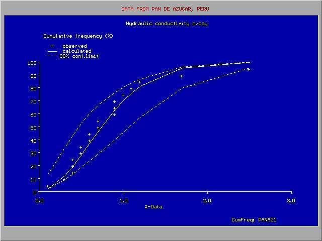
The picture shows a large variation of K -values measured with the augerhole method in an area of 100 ha. The ratio between the highest and lowest values is 25. The cumulative frequency distribution is lognormal and was made with the CumFreq program.

Transmissivity

The transmissivity is a measure of how much water can be transmitted horizontally, such as to a pumping well.

Transmissivity should not be confused with the similar word transmittance used in optics, meaning the fraction of incident light that passes through a sample.

An aquifer may consist of n soil layers. The transmissivity for horizontal flow T i of the i -th soil layer with a saturated thickness d i and horizontal hydraulic conductivity K i is:

T i = K i d i

Transmissivity is directly proportional to horizontal hydraulic conductivity K i and thickness d i . Expressing K i in m/day and d i in m, the transmissivity T i is found in units m²/day.
The total transmissivity T t of the aquifer is:

T t = ∑ T i where ∑ signifies the summation over all layers i = 1 , 2 , 3 , ⋯ , n .

The apparent horizontal hydraulic conductivity K A of the aquifer is:

K A = T t / D t

where D t , the total thickness of the aquifer, is D t = ∑ d i , with i = 1 , 2 , 3 , ⋯ , n .

The transmissivity of an aquifer can be determined from pumping tests.

Influence of the water table
When a soil layer is above the water table, it is not saturated and does not contribute to the transmissivity. When the soil layer is entirely below the water table, its saturated thickness corresponds to the thickness of the soil layer itself. When the water table is inside a soil layer, the saturated thickness corresponds to the distance of the water table to the bottom of the layer. As the water table may behave dynamically, this thickness may change from place to place or from time to time, so that the transmissivity may vary accordingly.
In a semi-confined aquifer, the water table is found within a soil layer with a negligibly small transmissivity, so that changes of the total transmissivity ( D t ) resulting from changes in the level of the water table are negligibly small.
When pumping water from an unconfined aquifer, where the water table is inside a soil layer with a significant transmissivity, the water table may be drawn down whereby the transmissivity reduces and the flow of water to the well diminishes.

Resistance

The resistance to vertical flow ( R i ) of the i -th soil layer with a saturated thickness d i and vertical hydraulic conductivity K v i is:

R i = d i / K v i

Expressing K v i in m/day and d i in m, the resistance ( R i ) is expressed in days.
The total resistance ( R t ) of the aquifer is:

R t = ∑ R i = ∑ d i / K v i

where ∑ signifies the summation over all layers: i = 1 , 2 , 3 , . . . , n .
The apparent vertical hydraulic conductivity ( K v A ) of the aquifer is:

K v A = D t / R t

where D t is the total thickness of the aquifer: D t = ∑ d i , with i = 1 , 2 , 3 , . . . , n .

The resistance plays a role in aquifers where a sequence of layers occurs with varying horizontal permeability so that horizontal flow is found mainly in the layers with high horizontal permeability while the layers with low horizontal permeability transmit the water mainly in a vertical sense.

Anisotropy

When the horizontal and vertical hydraulic conductivity ( K h i and K v i ) of the i -th soil layer differ considerably, the layer is said to be anisotropic with respect to hydraulic conductivity.
When the apparent horizontal and vertical hydraulic conductivity ( K h A and K v A ) differ considerably, the aquifer is said to be anisotropic with respect to hydraulic conductivity.
An aquifer is called semi-confined when a saturated layer with a relatively small horizontal hydraulic conductivity (the semi-confining layer or aquitard) overlies a layer with a relatively high horizontal hydraulic conductivity so that the flow of groundwater in the first layer is mainly vertical and in the second layer mainly horizontal.
The resistance of a semi-confining top layer of an aquifer can be determined from pumping tests.
When calculating flow to drains or to a well field in an aquifer with the aim to control the water table, the anisotropy is to be taken into account, otherwise the result may be erroneous.

Relative properties

Because of their high porosity and permeability, sand and gravel aquifers have higher hydraulic conductivity than clay or unfractured granite aquifers. Sand or gravel aquifers would thus be easier to extract water from (e.g., using a pumping well) because of their high transmissivity, compared to clay or unfractured bedrock aquifers.

Hydraulic conductivity has units with dimensions of length per time (e.g., m/s, ft/day and (gal/day)/ft² ); transmissivity then has units with dimensions of length squared per time. The following table gives some typical ranges (illustrating the many orders of magnitude which are likely) for K values.

Hydraulic conductivity (K) is one of the most complex and important of the properties of aquifers in hydrogeology as the values found in nature:

range over many orders of magnitude (the distribution is often considered to be lognormal),

vary a large amount through space (sometimes considered to be randomly spatially distributed, or stochastic in nature),

are directional (in general K is a symmetric second-rank tensor; e.g., vertical K values can be several orders of magnitude smaller than horizontal K values),

are scale dependent (testing a m³ of aquifer will generally produce different results than a similar test on only a cm³ sample of the same aquifer),

must be determined indirectly through field pumping tests, laboratory column flow tests or inverse computer simulation, (sometimes also from grain size analyses), and

are very dependent (in a non-linear way) on the water content, which makes solving the unsaturated flow equation difficult. In fact, the variably saturated K for a single material varies over a wider range than the saturated K values for all types of materials (see chart below for an illustrative range of the latter).

Ranges of values for natural materials

Table of saturated hydraulic conductivity (K) values found in nature

Values are for typical fresh groundwater conditions — using standard values of viscosity and specific gravity for water at 20 °C and 1 atm. See the similar table derived from the same source for intrinsic permeability values.

Source: modified from Bear, 1972