Hook length formula

Definitions and statement

Let λ = ( λ 1 , … , λ m ) be a partition of n . It is customary to interpret λ graphically as a Young diagram, namely a left-justified array of square cells with m rows and λ i cells in the i th row for each 1 ≤ i ≤ m . A standard Young tableau of shape λ is a Young diagram of shape λ in which each of the n cells contains a distinct integer between 1 and n (i.e., no repetition), such that each row and each column form increasing sequences. For each cell of the Young diagram in coordinates ( i , j ) (that is, the cell in the i th row and j th column), the hook H λ ( i , j ) is the set of cells ( a , b ) such that a = i and b ≥ j or a ≥ i and b = j . The hook-length h λ ( i , j ) is the number of cells in the hook H λ ( i , j ) .

Then the hook-length formula expresses the number of standard Young tableaux of shape λ , sometimes denoted by d λ , as

where the product is over all cells ( i , j ) of λ .

Example

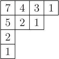
The figure on the right shows hook-lengths for all cells in the Young diagram λ of the partition
9 = 4 + 3 + 1 + 1. Then the number of standard Young tableaux d λ for this Young diagram can be computed as

History

There are other formulas for d λ , but the hook-length formula is particularly simple and elegant. The hook-length formula was discovered in 1954 by J. S. Frame, G. de B. Robinson, and R. M. Thrall by improving a less convenient formula expressing d λ in terms of a determinant. This earlier formula was deduced independently by G. Frobenius and A. Young in 1900 and 1902 respectively using algebraic methods. P. A. MacMahon found an alternate proof for the Young–Frobenius formula in 1916 using difference methods.

Despite the simplicity of the hook-length formula, the Frame–Robinson–Thrall proof is uninsightful and does not provide an intuitive argument as to why hooks appear in the formula. The search for a short, intuitive explanation befitting such a simple result gave rise to many alternate proofs for the hook-length formula. A. P. Hillman and R. M. Grassl gave the first proof that illuminates the role of hooks in 1976 by proving a special case of the Stanley hook-content formula, which is known to imply the hook-length formula. C. Greene, A. Nijenhuis, and H. S. Wilf found a probabilistic proof using the hook walk in which the hook lengths appear naturally in 1979. J. B. Remmel adapted the original Frame–Robinson–Thrall proof into the first bijective proof for the hook-length formula in 1982. A direct bijective proof was first discovered by D. S. Franzblau and D. Zeilberger in 1982. D. Zeilberger also converted the Greene–Nijenhuis–Wilf hook walk proof into a bijective proof in 1984. A simpler direct bijective proof was announced by Igor Pak and Alexander V. Stoyanovskii in 1992, and its complete proof was presented by the pair and Jean-Christophe Novelli in 1997.

Meanwhile, the hook-length formula has been generalized in several ways. R. M. Thrall found the analogue to the hook-length formula for shifted Young Tableaux in 1952. B. E. Sagan gave a shifted hook walk proof for the hook-length formula for shifted Young tableaux in 1980. B. E. Sagan and Y. N. Yeh proved the hook-length formula for binary trees using the hook walk in 1989.

Knuth's heuristic argument

The hook-length formula can be understood intuitively using the following heuristic, but incorrect, argument suggested by D. E. Knuth. Given that each element of a tableau is the smallest in its hook and filling the tableau shape at random, the probability that cell ( i , j ) will contain the minimum element of the corresponding hook is the reciprocal of the hook length. Multiplying these probabilities over all i and j gives the formula. This argument is fallacious since the events are not independent.

Knuth's argument is however correct for the enumeration of labellings on trees satisfying monotonicity properties analogous to those of a Young tableau. In this case, the 'hook' events in question are in fact independent events.

Probabilistic proof using the hook walk

This is a probabilistic proof found by C. Greene, A. Nijenhuis, and H. S. Wilf in 1979. Here is a sketch of the proof. Define

we would like to show that d λ = e λ . The first observation about d λ is

where μ ↑ λ denotes that μ are Young tableau obtained from λ by deleting one corner cell from λ . The sum is taken over all such μ . Here we are taking the convention that d ϕ = 1 , where ϕ denotes the empty diagram. The explanation for the above equation is that the maximal entry of the Young tableau of shape λ occurs at one of its corner cells. By deleting that cell we will obtain a Young tableau of shape μ . Since the number of Young tableau of shape μ is d μ , taking the sum over all such μ we get the equation.

Notice that we also have e ϕ = 1 . Therefore, it is enough to show that

and the result d λ = e λ then follows by induction. The above sum can also be viewed as a sum of probabilities by rewriting the equation to be shown as

We therefore need to show that the numbers e μ e λ define a probability measure on the set of Young diagrams μ (where μ ↑ λ ). This is done in a constructive way by defining a random walk, called the hook walk, on the cells of the Young diagram λ , which eventually selects one of the corner cells of λ (which are in bijection with diagrams μ for which μ ↑ λ ). The hook walk is defined by the following rules.

(1) Pick a cell uniformly at random from | λ | cells. Start the random walk from there.

(2) Successor of current cell ( i , j ) is chosen uniformly at random from the hook H λ ( i , j ) ∖ { ( i , j ) } .

(3) Continue until you reach at one of the corner cells, call it c .

Proposition: For any corner cell ( a , b ) of λ we have

where μ = λ ∖ { ( a , b ) } .

Once we have the above proposition, taking the sum over all possible corner cells c = ( a , b ) we have ∑ μ ↑ λ e μ e λ = 1 , as claimed.

Connection to representation theory

The hook-length formula is of great importance in the representation theory of the symmetric group S n , where the number d λ is known to be equal to the dimension of the complex irreducible representation V λ associated to λ , and is frequently denoted by dim ⁡ V λ , dim ⁡ λ or f λ .

Detailed discussion

The complex irreducible representations V λ of the symmetric group are indexed by partitions λ of n (for an explicit construction see Specht module) . Their characters are related to the theory of symmetric functions via the Hall inner product in the following formula

where s λ is the Schur function associated to λ and p τ ( w ) is the power-sum symmetric function of the partition τ ( w ) associated to the cycle decomposition of w . For example, if w = ( 154 ) ( 238 ) ( 6 ) ( 79 ) then τ ( w ) = ( 3 , 3 , 2 , 1 ) .

Since the identity permutation e has the form e = ( 1 ) ( 2 ) ⋯ ( n ) in cycle notation, τ ( e ) = 1 + 1 + ⋯ + 1 = 1 ( n ) . Then the formula says

Considering the expansion of Schur functions in terms of monomial symmetric functions using the Kostka numbers

the inner product with p 1 ( n ) = h 1 ( n ) is K λ 1 ( n ) , because ⟨ m μ , h ν ⟩ = δ μ ν . Note that K λ 1 ( n ) is equal to d λ . Hence

An immediate consequence of this is

The above equality is also a simple consequence of the Robinson–Schensted–Knuth correspondence.

The computation also shows that:

Which is the expansion of p 1 ( n ) in terms of Schur functions using the coefficients given by the inner product, because ⟨ s μ , s ν ⟩ = δ μ ν . The above equality can be proven also checking the coefficients of each monomial at both sides and using the Robinson–Schensted–Knuth correspondence or, more conceptually, looking at the decomposition of V ⊗ n by irreducible G L ( V ) modules, and taking characters. See Schur–Weyl duality.

Outline of the proof of the hook formula using Frobenius formula

By the above considerations

So that

where Δ ( x ) = ∏ i < j ( x i − x j ) is the Vandermonde determinant.

For a given partition λ = ( λ 1 , λ 2 , ⋯ , λ k ) define l i = λ i + k − i for i = 1 , 2 , ⋯ , k . For the following we need at least as many variables as rows in the partition, so from now on we work with n variables x 1 , ⋯ , x n .

Each term Δ ( x ) s λ is equal to

See Schur function. Since the vector ( l 1 , l 2 , ⋯ , l k ) is different for each partition, this means that the coefficient of x 1 l 1 ⋯ x k l k in Δ ( x ) p 1 ( n ) , denoted [ Δ ( x ) p 1 ( n ) ] l 1 , ⋯ , l k , is equal to f λ . This is known as the Frobenius Character Formula, which gives one of the earliest proofs. All that remains is tracking that coefficient with a mixture of cleverness and brute force: Multiplying

and

we conclude that the coefficient that we are looking for is

which can be written as

The latter sum is equal to the following determinant

which column reduces to the Vandermonde determinant, and we obtain the formula

Note that l i is the hook length of the first box in each row of the Young Diagram. Transforming this expression into the form n ! ∏ h λ ( i , j ) claimed by the hook-length formula is a fairly simple exercise in combinatorics: For any given i = 1 , 2 , … , k , one has to argue that l i ! = ( ∏ j > i ( l i − l j ) ) ⋅ ∏ c h λ ( c ) , where the latter product ranges over all cells c in the i -row of the Young diagram of λ .

Connection to longest increasing subsequences

The hook length formula also has important applications to the analysis of longest increasing subsequences in random permutations. If σ n denotes a uniformly random permutation of order n , L ( σ n ) denotes the maximal length of an increasing subsequence of σ n , and ℓ n denotes the expected (average) value of L ( σ n ) , Anatoly Vershik and Sergei Kerov and independently Benjamin F. Logan and Lawrence A. Shepp showed that when n is large, ℓ n is approximately equal to 2 n . This answers a question originally posed by Stanislaw Ulam. The proof is based on translating the question via the Robinson–Schensted correspondence to a problem about the limiting shape of a random Young tableau chosen according to Plancherel measure. Since the definition of Plancherel measure involves the quantity d λ , the hook length formula can then be used to perform an asymptotic analysis of the limit shape and thereby also answer the original question.

The ideas of Vershik–Kerov and Logan–Shepp were later refined by Jinho Baik, Percy Deift and Kurt Johansson, who were able to achieve a much more precise analysis of the limiting behavior of the maximal increasing subsequence length, proving an important result now known as the Baik–Deift–Johansson theorem. Their analysis again makes crucial use of the fact that d λ has a number of good formulas, although instead of the hook length formula it made use of one of the determinantal expressions.

Related formulas

The formula for the number of Young tableau of a given shape was originally derived from the Frobenius determinant formula in connection to representation theory. If the shape of a Young diagram is given by the row lengths n 1 , … , n m , then the number of tableau with that shape is given by

Hook lengths can also be used to give a product representation to the generating function for the number of reverse plane partitions of a given shape. If λ is a partition of some integer p, a reverse plane partition of n with shape λ is obtained by filling in the boxes in the Young diagram with non-negative integers such that the entries add to n and are non-decreasing along each row and down each column. The hook lengths h 1 , … , h p can be defined as with Young tableau. If π_n denotes the number of reverse plane partitions of n with shape λ, then the generating function can be written as

Stanley discovered another formula for the same generating function. In general, if A is any poset with n elements, the generating function for reverse A -partitions is

where P ( x ) is a polynomial such that P ( 1 ) is the number of natural labelings of A .

In the case of a partition λ , we are considering the poset in its cells given by the relation

So a natural labeling is simply a standard Young tableau, i.e. P ( 1 ) = f λ

Yet another proof of the hook length formula

Combining the two formulas for the generating functions we have

Both sides converge inside the disk of radius one and the following expression makes sense for | x | < 1

It would be violent to plug in 1, but the right hand side is a continuous function inside the unit disk and a polynomial is continuous everywhere so at least we can say

Finally, applying L'Hopital's rule n times yields the hook length formula

Specialization of Schur functions

Specializing the schur functions to the variables 1 , t , t 2 , t 3 , ⋯ there is the formula

The number n ( λ ) is defined as

where λ ′ is the conjugate partition

Skew shape formula

There is a generalization of this formula for skew shapes,

where the sum is taken over excited diagrams of shape λ and boxes distributed according to μ .

A formula for the Catalan numbers

The Catalan numbers are ubiquitous in enumerative combinatorics. Not surprisingly, they are also part of this story:

Lets briefly mention why. When doing a Dyck path we may go up (U) or down (D). So for any Dyck path of length n consider the tableaux of shape ( n , n ) such that the first row is given by the numbers i such that the i -th step was up and in the second row given by the positions in which it goes down. For example, UUDDUD correspond to the tableaux with rows 125 and 346.

The hook formula gives another way of getting a closed formula for the Catalan numbers