
 | ||
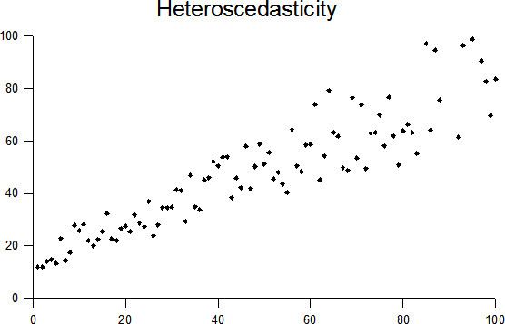
In statistics, a collection of random variables is heteroscedastic (or heteroskedastic; from Ancient Greek hetero “different” and skedasis “dispersion”) if there are sub-populations that have different variabilities from others. Here "variability" could be quantified by the variance or any other measure of statistical dispersion. Thus heteroscedasticity is the absence of homoscedasticity.
Contents
The existence of heteroscedasticity is a major concern in the application of regression analysis, including the analysis of variance, as it can invalidate statistical tests of significance that assume that the modelling errors are uncorrelated and uniform—hence that their variances do not vary with the effects being modeled. For instance, while the ordinary least squares estimator is still unbiased in the presence of heteroscedasticity, it is inefficient because the true variance and covariance are underestimated. Similarly, in testing for differences between sub-populations using a location test, some standard tests assume that variances within groups are equal.
Because heteroscedasticity concerns expectations of the second moment of the errors, its presence is referred to as misspecification of the second order.
Definition
Suppose there is a sequence of random variables
When using some statistical techniques, such as ordinary least squares (OLS), a number of assumptions are typically made. One of these is that the error term has a constant variance. This might not be true even if the error term is assumed to be drawn from identical distributions.
For example, the error term could vary or increase with each observation, something that is often the case with cross-sectional or time series measurements. Heteroscedasticity is often studied as part of econometrics, which frequently deals with data exhibiting it. While the influential 1980 paper by Halbert White used the term "heteroskedasticity" rather than "heteroscedasticity", the latter spelling has been employed more frequently in later works.
The econometrician Robert Engle won the 2003 Nobel Memorial Prize for Economics for his studies on regression analysis in the presence of heteroscedasticity, which led to his formulation of the autoregressive conditional heteroscedasticity (ARCH) modeling technique.
Consequences
One of the assumptions of the classical linear regression model is that there is no heteroscedasticity. Breaking this assumption means that the Gauss–Markov theorem does not apply, meaning that OLS estimators are not the Best Linear Unbiased Estimators (BLUE) and their variance is not the lowest of all other unbiased estimators. Heteroscedasticity does not cause ordinary least squares coefficient estimates to be biased, although it can cause ordinary least squares estimates of the variance (and, thus, standard errors) of the coefficients to be biased, possibly above or below the true or population variance. Thus, regression analysis using heteroscedastic data will still provide an unbiased estimate for the relationship between the predictor variable and the outcome, but standard errors and therefore inferences obtained from data analysis are suspect. Biased standard errors lead to biased inference, so results of hypothesis tests are possibly wrong. For example, if OLS is performed on a heteroscedastic data set, yielding biased standard error estimation, a researcher might fail to reject a null hypothesis at a given significance level, when that null hypothesis was actually uncharacteristic of the actual population (making a type II error).
Under certain assumptions, the OLS estimator has a normal asymptotic distribution when properly normalized and centered (even when the data does not come from a normal distribution). This result is used to justify using a normal distribution, or a chi square distribution (depending on how the test statistic is calculated), when conducting a hypothesis test. This holds even under heteroscedasticity. More precisely, the OLS estimator in the presence of heteroscedasticity is asymptotically normal, when properly normalized and centered, with a variance-covariance matrix that differs from the case of homoscedasticity. In 1980, White proposed a consistent estimator for the variance-covariance matrix of the asymptotic distribution of the OLS estimator. This validates the use of hypothesis testing using OLS estimators and White's variance-covariance estimator under heteroscedasticity.
Heteroscedasticity is also a major practical issue encountered in ANOVA problems. The F test can still be used in some circumstances.
However, it has been said that students in econometrics should not overreact to heteroscedasticity. One author wrote, "unequal error variance is worth correcting only when the problem is severe." In addition, another word of caution was in the form, "heteroscedasticity has never been a reason to throw out an otherwise good model." With the advent of heteroscedasticity-consistent standard errors allowing for inference without specifying the conditional second moment of error term, testing conditional homoscedasticity is not as important as in the past.
For any non-linear model (for instance Logit and Probit models), however, heteroscedasticity has more severe consequences: the maximum likelihood estimates of the parameters will be biased (in an unknown direction), as well as inconsistent (unless the likelihood function is modified to correctly take into account the precise form of heteroskedasticity). As pointed out by Greene, “simply computing a robust covariance matrix for an otherwise inconsistent estimator does not give it redemption. Consequently, the virtue of a robust covariance matrix in this setting is unclear.”
Detection
There are several methods to test for the presence of heteroscedasticity. Although tests for heteroscedasticity between groups can formally be considered as a special case of testing within regression models, some tests have structures specific to this case.
These tests consist of a test statistic (a mathematical expression yielding a numerical value as a function of the data), a hypothesis that is going to be tested (the null hypothesis), an alternative hypothesis, and a statement about the distribution of statistic under the null hypothesis.
Many introductory statistics and econometrics books, for pedagogical reasons, present these tests under the assumption that the data set in hand comes from a normal distribution. A great misconception is the thought that this assumption is necessary. Most of the methods of detecting heteroscedasticity outlined above can be modified for use even when the data do not come from a normal distribution. In many cases, this assumption can be relaxed, yielding a test procedure based on the same or similar test statistics but with the distribution under the null hypothesis evaluated by alternative routes: for example, by using asymptotic distributions which can be obtained from asymptotic theory, or by using resampling.
Fixes
There are four common corrections for heteroscedasticity. They are:
Examples
Heteroscedasticity often occurs when there is a large difference among the sizes of the observations.
Multivariate case
The study of heteroscedasticity has been generalized to the multivariate case, which deals with the covariances of vector observations instead of the variance of scalar observations. One version of this is to use covariance matrices as the multivariate measure of dispersion. Several authors have considered tests in this context, for both regression and grouped-data situations. Bartlett's test for heteroscedasticity between grouped data, used most commonly in the univariate case, has also been extended for the multivariate case, but a tractable solution only exists for 2 groups. Approximations exist for more than two groups, and they are both called Box's M test