Hammersley–Clifford theorem - Alchetron, the free social encyclopedia

The Hammersley–Clifford theorem is a result in probability theory, mathematical statistics and statistical mechanics, that gives necessary and sufficient conditions under which a positive probability distribution can be represented as a Markov network (also known as a Markov random field). It is the fundamental theorem of random fields. It states that a probability distribution that has a positive mass or density satisfies one of the Markov properties with respect to an undirected graph G if and only if it is a Gibbs random field, that is, its density can be factorized over the cliques (or complete subgraphs) of the graph.

The relationship between Markov and Gibbs random fields was initiated by Roland Dobrushin and Frank Spitzer in the context of statistical mechanics. The theorem is named after John Hammersley and Peter Clifford who proved the equivalence in an unpublished paper in 1971. Simpler proofs using the inclusion-exclusion principle were given independently by Geoffrey Grimmett, Preston and Sherman in 1973, with a further proof by Julian Besag in 1974.

Proof Outline

It is a trivial matter to show that a Gibbs random field satisfies every Markov property. As an example of this fact, see the following:

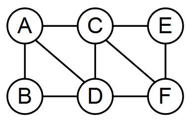
In the image to the right, a Gibbs random field over the provided graph has the form Pr ( A , B , C , D , E , F ) ∝ f 1 ( A , B , D ) f 2 ( A , C , D ) f 3 ( C , D , F ) f 4 ( C , E , F ) . If variables C and D are fixed, then the global Markov property requires that: A , B ⊥ E , F | C , D (see conditional independence), since C , D forms a barrier between A , B and E , F .

With C and D constant, Pr ( A , B , E , F | C , D ) ∝ [ f 1 ( A , B , D ) f 2 ( A , C , D ) ] ⋅ [ f 3 ( C , D , F ) f 4 ( C , E , F ) ] = g 1 ( A , B ) g 2 ( E , F ) where g 1 ( A , B ) = f 1 ( A , B , D ) f 2 ( A , C , D ) and g 2 ( E , F ) = f 3 ( C , D , F ) f 4 ( C , E , F ) . This implies that A , B ⊥ E , F | C , D .

To establish that every positive probability distribution that satisfies the local Markov property is also a Gibbs random field, the following lemma, which provides a means for combining different factorizations, needs to be proven:

Lemma 1

Let U denote the set of all random variables under consideration, and let Θ , Φ 1 , Φ 2 , … , Φ n ⊆ U and Ψ 1 , Ψ 2 , … , Ψ m ⊆ U denote arbitrary sets of variables. (Here, given an arbitrary set of variables X , X will also denote an arbitrary assignment to the variables from X .)

If

Pr ( U ) = f ( Θ ) ∏ i = 1 n g i ( Φ i ) = ∏ j = 1 m h j ( Ψ j )

for functions f , g 1 , g 2 , … g n and h 1 , h 2 , … , h m , then there exist functions h 1 ′ , h 2 ′ , … , h m ′ and g 1 ′ , g 2 ′ , … , g n ′ such that

Pr ( U ) = ( ∏ j = 1 m h j ′ ( Θ ∩ Ψ j ) ) ( ∏ i = 1 n g i ′ ( Φ i ) )

In other words, ∏ j = 1 m h j ( Ψ j ) provides a template for further factorization of f ( Θ ) .

Lemma 1 provides a means of combining two different factorizations of Pr ( U ) . The local Markov property implies that for any random variable x ∈ U , that there exists factors f x and f − x such that:

Pr ( U ) = f x ( x , ∂ x ) f − x ( U ∖ { x } )

where ∂ x are the neighbors of node x . Applying Lemma 1 repeatedly eventually factors Pr ( U ) into a product of clique potentials (see the image on the right).

End of Proof

References

Hammersley–Clifford theorem Wikipedia

(Text) CC BY-SA