
 | ||
A growing self-organizing map (GSOM) is a growing variant of the popular self-organizing map (SOM). The GSOM was developed to address the issue of identifying a suitable map size in the SOM. It starts with a minimal number of nodes (usually 4) and grows new nodes on the boundary based on a heuristic. By using the value called Spread Factor (SF), the data analyst has the ability to control the growth of the GSOM.
Contents
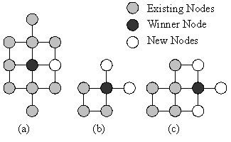
All the starting nodes of the GSOM are boundary nodes, i.e. each node has the freedom to grow in its own direction at the beginning. (Fig. 1) New Nodes are grown from the boundary nodes. Once a node is selected for growing all its free neighboring positions will be grown new nodes. The figure shows the three possible node growth options for a rectangular GSOM.
The algorithm
The GSOM process is as follows:
- Initialization phase:
- Initialize the weight vectors of the starting nodes (usually four) with random numbers between 0 and 1.
- Calculate the growth threshold (
G T ) for the given data set of dimensionD according to the spread factor (S F ) using the formulaG T = − D × ln ( S F )
- Growing Phase:
- Present input to the network.
- Determine the weight vector that is closest to the input vector mapped to the current feature map (winner), using Euclidean distance (similar to the SOM). This step can be summarized as: find
q ′ | v − w q ′ | ≤ | v − w q | ∀ q ∈ N wherev ,w are the input and weight vectors respectively,q is the position vector for nodes andN is the set of natural numbers. - The weight vector adaptation is applied only to the neighborhood of the winner and the winner itself. The neighborhood is a set of neurons around the winner, but in the GSOM the starting neighborhood selected for weight adaptation is smaller compared to the SOM (localized weight adaptation). The amount of adaptation (learning rate) is also reduced exponentially over the iterations. Even within the neighborhood, weights that are closer to the winner are adapted more than those further away. The weight adaptation can be described by
w j ( k + 1 ) = { w j ( k ) if j ∉ N k + 1 w j ( k ) + L R ( k ) × ( x k − w j ( k ) ) if j ∈ N k + 1 where the Learning Rate L R ( k ) ,k ∈ N is a sequence of positive parameters converging to zero ask → ∞ .w j ( k ) ,w j ( k + 1 ) are the weight vectors of the nodej before and after the adaptation andN k + 1 ( k + 1 ) th iteration. The decreasing value ofL R ( k ) in the GSOM depends on the number of nodes existing in the map at timek . - Increase the error value of the winner (error value is the difference between the input vector and the weight vectors).
- When
T E i > G T (whereT E i i andG T is the growth threshold). Grow nodes if i is a boundary node. Distribute weights to neighbors ifi is a non-boundary node. - Initialize the new node weight vectors to match the neighboring node weights.
- Initialize the learning rate (
L R ) to its starting value. - Repeat steps 2 – 7 until all inputs have been presented and node growth is reduced to a minimum level.
- Smoothing phase.
- Reduce learning rate and fix a small starting neighborhood.
- Find winner and adapt the weights of the winner and neighbors in the same way as in growing phase.
Applications
The GSOM can be used for many preprocessing tasks in Data mining, for Nonlinear dimensionality reduction, for approximation of principal curves and manifolds, for clustering and classification. It gives often the better representation of the data geometry than the SOM (see the classical benchmark for principal curves on the left).