
 | ||
In mathematics, Green's theorem gives the relationship between a line integral around a simple closed curve C and a double integral over the plane region D bounded by C. It is named after George Green and is the two-dimensional special case of the more general Kelvin–Stokes theorem.
Contents
Theorem
Let C be a positively oriented, piecewise smooth, simple closed curve in a plane, and let D be the region bounded by C. If L and M are functions of (x, y) defined on an open region containing D and have continuous partial derivatives there, then
where the path of integration along C is anticlockwise.
In physics, Green's theorem is mostly used to solve two-dimensional flow integrals, stating that the sum of fluid outflows from a volume is equal to the total outflow summed about an enclosing area. In plane geometry, and in particular, area surveying, Green's theorem can be used to determine the area and centroid of plane figures solely by integrating over the perimeter.
Proof when D is a simple region
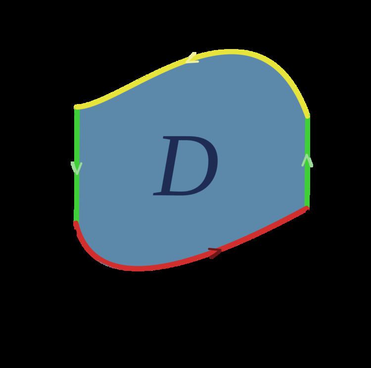
The following is a proof of half of the theorem for the simplified area D, a type I region where C1 and C3 are curves connected by vertical lines (possibly of zero length). A similar proof exists for the other half of the theorem when D is a type II region where C2 and C4 are curves connected by horizontal lines (again, possibly of zero length). Putting these two parts together, the theorem is thus proven for regions of type III (defined as regions which are both type I and type II). The general case can then be deduced from this special case by decomposing D into a set of type III regions.
If it can be shown that if
and
are true, then Green's theorem follows immediately for the region D. We can prove (1) easily for regions of type I, and (2) for regions of type II. Green's theorem then follows for regions of type III.
Assume region D is a type I region and can thus be characterized, as pictured on the right, by
where g1 and g2 are continuous functions on [a, b]. Compute the double integral in (1):
Now compute the line integral in (1). C can be rewritten as the union of four curves: C1, C2, C3, C4.
With C1, use the parametric equations: x = x, y = g1(x), a ≤ x ≤ b. Then
With C3, use the parametric equations: x = x, y = g2(x), a ≤ x ≤ b. Then
The integral over C3 is negated because it goes in the negative direction from b to a, as C is oriented positively (anticlockwise). On C2 and C4, x remains constant, meaning
Therefore,
Combining (3) with (4), we get (1) for regions of type I. A similar treatment yields (2) for regions of type II. Putting the two together, we get the result for regions of type III.
Relationship to Stokes' theorem
Green's theorem is a special case of the Kelvin–Stokes theorem, when applied to a region in the xy-plane:
We can augment the two-dimensional field into a three-dimensional field with a z component that is always 0. Write F for the vector-valued function
Kelvin–Stokes Theorem:
The surface
The expression inside the integral becomes
Thus we get the right side of Green's theorem
Green's theorem is also a straightforward result of the general Stokes' theorem using differential forms and exterior derivatives:
Relationship to the divergence theorem
Considering only two-dimensional vector fields, Green's theorem is equivalent to the two-dimensional version of the divergence theorem:
where
To see this, consider the unit normal
Start with the left side of Green's theorem:
Applying the two-dimensional divergence theorem with
Area calculation
Green's theorem can be used to compute area by line integral. The area of D is given by
Possible formulas for the area of D include: