
 | ||
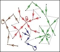
A gradient network is a directed subnetwork of an undirected "substrate" network in which each node has an associated scalar potential and one out-link that point to the node with the smallest (or largest) potential in its neighborhood, defined as the reunion of itself and its nearest neighbors on the substrate networks.
Contents
- Motivation
- In degree distribution of gradient networks
- The congestion on networks
- An efficient approach to control congestion
- References
Let us consider that transport takes place on a fixed network G = G(V,E) called the substrate graph. It has N nodes, V = {0, 1, ...,N − 1} and the set of edges E = { (i,j) | i,j ∈ V}. Given a node i, we can define its set of neighbors in G by Si(1) = {j ∈ V | (i,j)∈ E}.
Let us also consider a scalar field, h = {h0, .., hN−1} defined on the set of nodes V, so that every node i has a scalar value hi associated to it.
Gradient ∇hi on a network: ∇hi
Gradient network : ∇
In general, the scalar field depends on time, due to the flow, external sources and sinks on the network. Therefore, the gradient network ∇
Motivation
Real-world networks evolve to fulfill a main function, which is often to transport entities such as information, cars, power, water, etc. All these large-scale networks mentioned above are non-globally designed. They evolve and grow through local changes, through a natural selection-like dynamics. For example, if a router on the Internet is frequently congested and packets are lost or delayed due to that, it will get replaced by several interconnected new routers. Recent research investigate the connection between network topology and the flow efficiency of the transportation.
The flow is often generated or influenced by local gradients of a scalar, for example: electric current driven by a gradient of electric potential; in the information networks, properties of nodes will generate a bias in the way of information is transmitted from a node to its neighbors. This idea motivated the approach through gradient networks which studies flow efficiency on the network when the flow is driven by gradients of a scalar field distributed on the network
In-degree distribution of gradient networks
In a gradient network, in-degree of a node i, ki (in) is the number of gradient edges pointing into i, and the in-degree distribution
When the substrate G is random graph, and each pair of nodes is connected with probability P, the scalars hi are i.i.d. (independent identically distributed) the exact expression for R(l) is given by
In the limit N →∞ and P → 0, the degree distribution becomes the power law
This shows in this limit, the gradient network of random network is scale-free. If the subtstrate network G is scale-free, like BA model, then the gradient network also follow the power-law with the same exponent as those of G.
The congestion on networks
The fact that topology of substrate network influence the level of congestion can be illustrated by simple example(Fig.6.) as following: if the network has a star-like structure, then at the central node, the flow would congeste because the central node should handle all flow from others nodes. On the contrary, if the network has a ring-like structure, since every node take same role for transportation there is no traffic jam of flow.
Under assumption that the flow is generated by gradients in the network, characterize efficiency of flow on networks can be characterized through the jamming factor(or congestion factor) defined as:
where Nreceive is the number of nodes that receive gradient flow and Nsend is the number of nodes that send the flow. The value of J is in the range between 0 and 1. J = 0 means no congestion, and J = 1 corresponds to maximal congestion. In the limit N → ∞,and the probability with which two arbitrary nodes are connected is constant, for random network, the congestion factor becomes
This result show that random networks are maximally congested in that limit. On the contrary, for scale-free network, J is always a constant for any N. This conclusion means scale-free networks are not prone to maximal jamming.
An efficient approach to control congestion
A key problem in communication networks is to understand how to control congestion and maintain a normal and efficient functioning of the networks. Zonghua Liu et al. studied the network congestion and get the result that congestions are more likely to take place at the nodes with high degrees in networks (See Fig. 8), and an efficient approach of selectively enhancing the message-process capability of a small fraction(e.g. 3%) of nodes is shown to perform just as well as enhancing the capability of all nodes.(See Fig. 9)