Gauss–Newton algorithm

Description

Given m functions r = (r₁, …, r_m) (often called residuals) of n variables β = (β₁, …, β_n), with m ≥ n, the Gauss–Newton algorithm iteratively finds the value of the variables which minimizes the sum of squares

Starting with an initial guess β ( 0 ) for the minimum, the method proceeds by the iterations

where, if r and β are column vectors, the entries of the Jacobian matrix are

and the symbol T denotes the matrix transpose.

If m = n, the iteration simplifies to

which is a direct generalization of Newton's method in one dimension.

In data fitting, where the goal is to find the parameters β such that a given model function y = f(x, β) best fits some data points (x_i, y_i), the functions r_i are the residuals

Then, the Gauss-Newton method can be expressed in terms of the Jacobian J_f of the function f as

Example

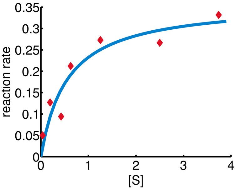
In this example, the Gauss–Newton algorithm will be used to fit a model to some data by minimizing the sum of squares of errors between the data and model's predictions.

In a biology experiment studying the relation between substrate concentration [S] and reaction rate in an enzyme-mediated reaction, the data in the following table were obtained.

It is desired to find a curve (model function) of the form

that fits best the data in the least squares sense, with the parameters V max and K M to be determined.

Denote by x i and y i the value of [S] and the rate from the table, i = 1 , … , 7. Let β 1 = V max and β 2 = K M . We will find β 1 and β 2 such that the sum of squares of the residuals

is minimized.

The Jacobian J r of the vector of residuals r i in respect to the unknowns β j is an 7 × 2 matrix with the i -th row having the entries

Starting with the initial estimates of β 1 = 0.9 and β 2 = 0.2 , after five iterations of the Gauss–Newton algorithm the optimal values β ^ 1 = 0.362 and β ^ 2 = 0.556 are obtained. The sum of squares of residuals decreased from the initial value of 1.445 to 0.00784 after the fifth iteration. The plot in the figure on the right shows the curve determined by the model for the optimal parameters versus the observed data.

Convergence properties

It can be shown that the increment Δ is a descent direction for S, and, if the algorithm converges, then the limit is a stationary point of S. However, convergence is not guaranteed, not even local convergence as in Newton's method, or convergence under the usual Wolfe conditions .

The rate of convergence of the Gauss–Newton algorithm can approach quadratic. The algorithm may converge slowly or not at all if the initial guess is far from the minimum or the matrix J r T J r is ill-conditioned. For example, consider the problem with m = 2 equations and n = 1 variable, given by

The optimum is at β = 0 . (Actually the optimum is at β = − 1 for λ = 2 , because S ( 0 ) = 1 2 + ( − 1 ) 2 = 2 , but S ( − 1 ) = 0 .) If λ = 0 then the problem is in fact linear and the method finds the optimum in one iteration. If |λ| < 1 then the method converges linearly and the error decreases asymptotically with a factor |λ| at every iteration. However, if |λ| > 1, then the method does not even converge locally.

Derivation from Newton's method

In what follows, the Gauss–Newton algorithm will be derived from Newton's method for function optimization via an approximation. As a consequence, the rate of convergence of the Gauss–Newton algorithm can be quadratic under certain regularity conditions. In general (under weaker conditions), the convergence rate is linear.

The recurrence relation for Newton's method for minimizing a function S of parameters, β , is

where g denotes the gradient vector of S and H denotes the Hessian matrix of S. Since S = ∑ i = 1 m r i 2 , the gradient is given by

Elements of the Hessian are calculated by differentiating the gradient elements, g j , with respect to β k

The Gauss–Newton method is obtained by ignoring the second-order derivative terms (the second term in this expression). That is, the Hessian is approximated by

where J i j = ∂ r i ∂ β j are entries of the Jacobian J_r. The gradient and the approximate Hessian can be written in matrix notation as

These expressions are substituted into the recurrence relation above to obtain the operational equations

Convergence of the Gauss–Newton method is not guaranteed in all instances. The approximation

that needs to hold to be able to ignore the second-order derivative terms may be valid in two cases, for which convergence is to be expected.

1. The function values r i are small in magnitude, at least around the minimum.
2. The functions are only "mildly" non linear, so that ∂ 2 r i ∂ β j ∂ β k is relatively small in magnitude.

Improved versions

With the Gauss–Newton method the sum of squares of the residuals S may not decrease at every iteration. However, since Δ is a descent direction, unless S ( β s ) is a stationary point, it holds that S ( β s + α Δ ) < S ( β s ) for all sufficiently small α > 0 . Thus, if divergence occurs, one solution is to employ a fraction, α , of the increment vector, Δ in the updating formula:

In other words, the increment vector is too long, but it points in "downhill", so going just a part of the way will decrease the objective function S. An optimal value for α can be found by using a line search algorithm, that is, the magnitude of α is determined by finding the value that minimizes S, usually using a direct search method in the interval 0 < α < 1 .

In cases where the direction of the shift vector is such that the optimal fraction, α , is close to zero, an alternative method for handling divergence is the use of the Levenberg–Marquardt algorithm, also known as the "trust region method". The normal equations are modified in such a way that the increment vector is rotated towards the direction of steepest descent,

where D is a positive diagonal matrix. Note that when D is the identity matrix I and λ → + ∞ , then λ Δ = λ ( J T J + λ I ) − 1 ( − J T r ) = ( I − J T J / λ + ⋯ ) ( − J T r ) → − J T r , therefore the direction of Δ approaches the direction of the negative gradient − J T r .

The so-called Marquardt parameter, λ , may also be optimized by a line search, but this is inefficient as the shift vector must be re-calculated every time λ is changed. A more efficient strategy is this. When divergence occurs increase the Marquardt parameter until there is a decrease in S. Then, retain the value from one iteration to the next, but decrease it if possible until a cut-off value is reached when the Marquardt parameter can be set to zero; the minimization of S then becomes a standard Gauss–Newton minimization.

Large-scale optimization

For large scale optimization, the Gauss-Newton method is of special interest because it is often (though certainly not always) true that the matrix J r is more sparse than the approximate Hessian J r T J r . In such cases, the step calculation itself will typically need to be done with an approximate iterative method appropriate for large and sparse problems, such as the conjugate gradient method.

In order to make this kind of approach work, one needs at minimum an efficient method for computing the product

for some vector p. With sparse matrix storage, it is in general practical to store the rows of J r in a compressed form (eg, without zero entries), making a direct computation of the above product tricky due to the transposition. However, if one defines c_i as row i of the matrix J r , the following simple relation holds

so that every row contributes additively and independently to the product. In addition to respecting a practical sparse storage structure, this expression is well suited for parallel computations. Note that every row c_i is the gradient of the corresponding residual r_i; with this in mind, the formula above emphasizes the fact that residuals contribute to the problem independently of each other.

Related algorithms

In a quasi-Newton method, such as that due to Davidon, Fletcher and Powell or Broyden–Fletcher–Goldfarb–Shanno (BFGS method) an estimate of the full Hessian, ∂ 2 S ∂ β j ∂ β k , is built up numerically using first derivatives ∂ r i ∂ β j only so that after n refinement cycles the method closely approximates to Newton's method in performance. Note that quasi-Newton methods can minimize general real-valued functions, whereas Gauss-Newton, Levenberg-Marquardt, etc. fits only to nonlinear least-squares problems.

Another method for solving minimization problems using only first derivatives is gradient descent. However, this method does not take into account the second derivatives even approximately. Consequently, it is highly inefficient for many functions, especially if the parameters have strong interactions.