Folded Reed–Solomon code

History

One of the ongoing challenges in Coding Theory is to have error correcting codes achieve an optimal trade-off between (Coding) Rate and Error-Correction Radius. Though this may not be possible to achieve practically (due to Noisy Channel Coding Theory issues), quasi optimal tradeoffs can be achieved theoretically.

Prior to Folded Reed–Solomon codes being devised, the best Error-Correction Radius achieved was 1 − R , by Reed–Solomon codes for all rates R .

An improvement upon this 1 − R bound was achieved by Parvaresh and Vardy for rates R < 1 16 .

For R → 0 the Parvaresh–Vardy algorithm can decode a fraction 1 − O ( R log ⁡ ( 1 / R ) ) of errors.

Folded Reed–Solomon Codes improve on these previous constructions, and can be list decoded in polynomial time for a fraction ( 1 − R − ε ) of errors for any constant ε > 0 .

Definition

f ( X ) ↦ [ f ( 1 ) f ( γ ) ⋮ f ( γ m − 1 ) ] , [ f ( γ m ) f ( γ m + 1 ) ⋮ f ( γ 2 m − 1 ) ] , … , [ f ( γ n − m ) f ( γ n − m + 1 ) ⋮ f ( γ n − 1 ) ]

Consider a Reed–Solomon [ n = q − 1 , k ] q code of length n and dimension k and a folding parameter m ≥ 1 . Assume that m divides n .

Mapping for Reed–Solomon codes like this:

f ↦ ⟨ f ( 1 ) , f ( γ 1 ) , f ( γ 2 ) , … , f ( γ n − 1 ) ⟩

where γ ∈ F q is a primitive element in

F q = { 0 , 1 , γ , γ 2 , … , γ n − 1 } .

The m folded version of Reed Solomon code C , denoted F R S F , γ , m , k is a code of block length N = n / m over F m . F R S F , γ , m , k are just [ q − 1 , k ] Reed Solomon codes with m consecutive symbols from RS codewords grouped together.

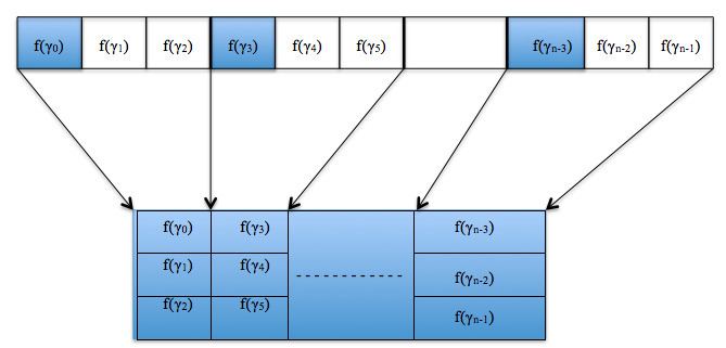
Graphic description

The above definition is made more clear by means of the diagram with m = 3 , where m is the folding parameter.

The message is denoted by f ( X ) , which when encoded using Reed–Solomon encoding, consists of values of f at x 0 , x 1 , x 2 , … , x n − 1 , where x i = γ i .

Then bundling is performed in groups of 3 elements, to give a codeword of length n / 3 over the alphabet F q 3 .

Something to be observed here is that the folding operation demonstrated does not change the rate R of the original Reed–Solomon code.

To prove this, consider a linear [ n , k , d ] q code, of length n , dimension k and distance d . The m folding operation will make it a [ n m , k m , d m ] q m code. By this, the rate R = n k will be the same.

Folded Reed–Solomon codes and the singleton bound

According to the asymptotic version of the singleton bound, it is known that the relative distance δ , of a code must satisfy R ⩽ 1 − δ + o ( 1 ) where R is the rate of the code. As proved earlier, since the rate R is maintained, the relative distance δ ⩾ 1 − R also meets the Singleton bound.

Why folding might help?

Folded Reed–Solomon codes are basically the same as Reed Solomon codes, just viewed over a larger alphabet. To show how this might help, consider a folded Reed–Solomon code with m = 3 . Decoding a Reed–Solomon code and folded Reed–Solomon code from the same fraction of errors ρ are tasks of almost of the same computational intensity: one can unfold the received word of the folded Reed–Solomon code, treat it as an received word of the original Reed–Solomon code, and run the Reed–Solomon list decoding algorithm on it. Obviously, this list will contain all the folded Reed–Solomon codewords within distance ρ of the received word, along with some extras, which we can expurgate.

Also, decoding a folded Reed–Solomon code is an easier task. Suppose we want to correct a third of errors. The decoding algorithm chosen must correct an error pattern that corrects every third symbol in the Reed–Solomon encoding. But after folding, this error pattern will corrupt all symbols over F q 3 and will eliminate the need for error correction. This propagation of errors is indicated by the blue color in the graphical description. This proves that the for a fixed fraction of errors ρ , the folding operation reduces the channel's flexibility to distribute errors, which in turn leads to a reduction in the number of error patterns that need to be corrected.

How folded Reed–Solomon (FRS) codes and Parvaresh Vardy (PV) codes are related

We can relate Folded Reed Solomon codes with Parvaresh Vardy codes which encodes a polynomial f of degree k with polynomials f 0 = f , f 1 , … , f s − 1 ( s ⩾ 2 ) where f i ( X ) = f i − 1 ( X ) d mod E ( X ) where E ( X ) is an irreducible polynomial. While choosing irreducible polynomial E ( X ) = X q − γ and parameter d we should check if every polynomial f of degree at most k satisfies f ( γ X ) = f ( X ) d mod E ( X ) since f ( γ X ) is just the shifted counterpart of f ( X ) where γ is the primitive element in F q . Thus folded RS code with bundling together code symbols is PV code of order s = m for the set of evaluation points

{ 1 , γ , γ 2 m , … , γ ( n m − 1 ) m } .

If we compare the folded RS code to a PV code of order 2 for the set of evaluation points

{ 1 , γ , … , γ m − 2 , γ m , γ m + 1 , … , γ 2 m − 2 , … , γ n − m , γ n − m + 1 , … , γ n − 2 }

we can see that in PV encoding of f , for every 0 ≤ i ≤ n / m − 1 and every 0 < j < m − 1 , f ( γ m i + j ) appears at f ( γ m i + j ) and f 1 ( γ − 1 γ m i + j ) ,

unlike in the folded FRS encoding in which it appears only once. Thus, the PV and folded RS codes have same information but only the rate of FRS is bigger by a factor of 2 ( m − 1 ) / m and hence the list decoding radius trade-off is better for folded RS code by just using the list decodability of the PV codes. The plus point is in choosing FRS code in a way that they are compressed forms of suitable PV code with similar error correction performance with better rate than corresponding PV code. One can use this idea to construct a folded RS codes of rate R that are list decodable up to radius approximately 1 − R s / [ s + 1 ] for s ≥ 1 . [2]

Brief overview of list-decoding folded Reed–Solomon codes

A list decoding algorithm which runs in quadratic time to decode FRS code up to radius 1 − R − ε is presented by Guruswami. The algorithm essentially has three steps namely the interpolation step in which welch berlekamp style interpolation is used to interpolate the non-zero polynomial

Q ( X , Y 1 , Y 2 , … , Y s ) = A 0 ( X ) + A 1 ( X ) Y 1 + A 2 ( X ) Y 2 + ⋯ + A s ( X ) Y s ,

after which all the polynomials f ∈ F q [ X ] with degree k − 1 satisfying the equation derived in interpolation are found. In the third step the actual list of close-by codewords are known by pruning the solution subspace which takes q s time.

Linear-algebraic list decoding algorithm

Guruswami presents a n Ω ( 1 / ε 2 ) time list decoding algorithm based on linear-algebra, which can decode folded Reed–Solomon code up to radius 1 − R − ε with a list-size of n O ( 1 / ε 2 ) . There are three steps in this algorithm: Interpolation Step, Root Finding Step and Prune Step. In the Interpolation step it will try to find the candidate message polynomial f ( x ) by solving a linear system. In the Root Finding step, it will try to find the solution subspace by solving another linear system. The last step will try to prune the solution subspace gained in the second step. We will introduce each step in details in the following.

Step 1: The interpolation step

It is a Welch–Berlekamp-style interpolation (because it can be viewed as the higher-dimensional generalization of the Welch–Berlekamp algorithm). Suppose we received a codeword y of the m -folded Reed–Solomon code as shown below

( [ y 0 y 1 y 2 ⋯ y m − 1 ] , [ y m y m + 1 y m + 2 ⋯ y 2 m − 1 ] , ⋯ , [ y n − m y n − m + 1 y n − m + 2 ⋯ y n − 1 ] )

We interpolate the nonzero polynomial

Q ( X , Y 1 , … , Y s ) = A 0 ( X ) + A 1 ( X ) Y 1 + ⋯ + A s ( X ) Y s , { deg ⁡ ( A i ) ⩽ D 1 ⩽ i ⩽ s deg ⁡ ( A 0 ) ⩽ D + k − 1

by using a carefully chosen degree parameter D .

D = ⌊ N ( m − s + 1 ) − k + 1 s + 1 ⌋

So the interpolation requirements will be

Q ( γ i m + j , y i m + j , y i m + j + 1 , … , y i m + j + s − 1 ) = 0 , for i = 0 , 1 , … , n m − 1 , j = 0 , 1 , … , m − s .

Then the number of monomials in Q ( X , Y 1 , … , Y s ) is

( D + 1 ) s + D + k = ( D + 1 ) ( s + 1 ) + k − 1 > N ( m − s + 1 )

Because the number of monomials in Q ( X , Y 1 , … , Y s ) is greater than the number of interpolation conditions. We have below lemma

Lemma 1. 0 ≠ Q ∈ F q [ X , Y 1 , … , Y s ] satisfying the above interpolation condition can be found by solving a homogeneous linear system over F q with at most N m constraints and variables. Moreover this interpolation can be performed in O ( N m log 2 ⁡ ( N m ) log ⁡ log ⁡ ( N m ) ) operations over F q .

This lemma shows us that the interpolation step can be done in near-linear time.

For now, we have talked about everything we need for the multivariate polynomial Q ( X , Y 1 , … , Y s ) . The remaining task is to focus on the message polynomials f ( X ) .

Lemma 2. If a candidate message polynomial f ( X ) ∈ F [ X ] is a polynomial of degree at most k − 1 whose Folded Reed-Solomon encoding agrees with the received word y in at least t columns with t > D + k − 1 m − s + 1 , then Q ( X , f ( X ) , f ( γ X ) , … , f ( γ s − 1 X ) ) = 0.

Here "agree" means that all the m values in a column should match the corresponding values in codeword y .

This lemma shows us that any such polynomial Q ( X , Y 1 , … , Y s ) presents an algebraic condition that must be satisfied for those message polynomials f ( x ) that we are interested in list decoding.

Combining Lemma 2 and parameter D , we have

t ( m − s + 1 ) > N ( m − s + 1 ) + s ( k − 1 ) s + 1

Further we can get the decoding bound

t ⩾ N s + 1 + s s + 1 ⋅ k m − s + 1 = N ( 1 s + 1 + s s + 1 ⋅ m R m − s + 1 )

We notice that the fractional agreement is

1 s + 1 + s s + 1 ⋅ m R m − s + 1

Step 2: The root-finding step

During this step, our task focus on how to find all polynomials f ∈ F q [ X ] with degree no more than k − 1 and satisfy the equation we get from Step 1, namely

A 0 ( X ) + A 1 ( X ) f ( X ) + A 2 ( X ) f ( γ X ) + ⋯ + A s ( X ) f ( γ s − 1 X ) = 0

Since the above equation forms a linear system equations over F q in the coefficients f 0 , f 1 , … , f k − 1 of the polynomial

f ( X ) = f 0 + f 1 X + ⋯ + f k − 1 X k − 1 ,

the solutions to the above equation is an affine subspace of F q k . This fact is the key point that gives rise to an efficient algorithm - we can solve the linear system.

It is natural to ask how large is the dimension of the solution? Is there any upper bound on the dimension? Having an upper bound is very important in constructing an efficient list decoding algorithm because one can simply output all the codewords for any given decoding problem.

Actually it indeed has an upper bound as below lemma argues.

Lemma 3. If the order of γ is at least k (in particular when γ is primitive), then the dimension of the solution is at most s − 1 .

This lemma shows us the upper bound of the dimension for the solution space.

Finally, based on the above analysis, we have below theorem

Theorem 1. For the folded Reed–Solomon code F R S q ( m ) [ n , k ] of block length N = n m and rate R = k n , the following holds for all integers s , 1 ⩽ s ⩽ m . Given a received word y ∈ ( F q m ) N , in O ( ( N m log ⁡ q ) 2 ) time, one can find a basis for a subspace of dimension at most s − 1 that contains all message polynomials f ∈ F q [ X ] of degree less than k whose FRS encoding differs from y in at most a fraction s s + 1 ( 1 − m R m − s + 1 ) of the N codeword positions.

When s = m = 1 , we notice that this reduces to a unique decoding algorithm with up to a fraction ( 1 − R ) / 2 of errors. In other words, we can treat unique decoding algorithm as a specialty of list decoding algorithm. The quantity is about n O ( 1 / ε ) for the parameter choices that achieve a list decoding radius of 1 − R − ε .

Theorem 1 tells us exactly how large the error radius would be.

Now we finally get the solution subspace. However, there is still one problem standing. The list size in the worst case is n Ω ( 1 / ε ) . But the actual list of close-by codewords is only a small set within that subspace. So we need some process to prune the subspace to narrow it down. This prune process takes q s time in the worst case. Unfortunately it is not known how to improve the running time because we do not know how to improve the bound of the list size for folded Reed-Solomon code.

Things get better if we change the code by carefully choosing a subset of all possible degree k − 1 polynomials as messages, the list size shows to be much smaller while only losing a little bit in the rate. We will talk about this briefly in next step.

Step 3: The prune step

By converting the problem of decoding a folded Reed–Solomon code into two linear systems, one linear system that is used for the interpolation step and another linear system to find the candidate solution subspace, the complexity of the decoding problem is successfully reduced to quadratic. However, in the worst case, the bound of list size of the output is pretty bad.

It was mentioned in Step 2 that if one carefully chooses only a subset of all possible degree k − 1 polynomials as messages, the list size can be much reduced. Here we will expand our discussion.

To achieve this goal, the idea is to limit the coefficient vector ( f 0 , f 1 , … , f k − 1 ) to a special subset ν ⊆ F q k , which satisfies below two conditions:

Condition 1. The set ν must be large enough ( | ν | ≥ q ( 1 − ε ) k ).

This is to make sure that the rate will be at most reduced by factor of ( 1 − ε ) .

Condition 2. The set ν should have low intersection with any subspace S of dimension s satisfying S ⊂ F q k and | S ∩ ν | ⩽ L . Such a subset is called subspace-evasive subset.

The bound for the list size at worst case is n Ω ( 1 / ε ) , and it can be reduced to a relative small bound O ( 1 / ε 2 ) by using subspace-evasive subsets.

During this step, as it has to check each element of the solution subspace that we get from Step 2, it takes q s time in the worst case ( s is the dimension of the solution subspace).

Dvir and Lovett improved the result based on the work of Guruswami, which can reduce the list size to a constant.

Here is only presented the idea that is used to prune the solution subspace. For the details of the prune process, please refer to papers by Guruswami, Dvir and Lovett, which are listed in the reference.

Summary

If we don't consider the Step 3, this algorithm can run in quadratic time. A summary for this algorithm is listed below.