Finite and Deterministic Discrete Event System Specification

History

FD-DEVS was originally named as ``Schedule-Controlable DEVS`` [Hwang05] and designed to support verification analysis of its networks which had been an open problem of DEVS formalism for 30 years. In addition, it was also designated to resolve the so-called ``OPNA`` problem of SP-DEVS. From the viewpoint of Classic DEVS, FD-DEVS has three restrictions

1. finiteness of event sets and state set,
2. the lifespan of a state can be scheduled by a rational number or infinity, and
3. the internal schedule can be either preserved or updated by an input event.

The third restriction can be also seen as a relaxation from SP-DEVS where the schedule is always preserved by any input events. Due to this relaxation there is no longer OPNA problem, but there is also one limitation that a time-line abstraction which can be used for abstracting elapsed times of SP-DEVS networks is no longer useful for FD-DEVS network [Hwang05]. But another time abstraction method [Dill89] which was invented by Prof. D. Dill can be applicable to obtain a finite-vertex reachability graph for FD-DEVS networks.

Ping-pong game

Consider a single ping-pong match in which there are two players. Each player can be modeled by FD-DEVS such that the player model has an input event ?receive and an output event !send, and it has two states: Send and Wait. Once the player gets into ``Send``, it will generates ``!send`` and go back to ``Wait`` after the sending time which is 0.1 time unit. When staying at ``Wait`` and if it gets ``?receive``, it changes into ``Send`` again. In other words, the player model stays at ``Wait`` forever unless it gets ``?receive``.

To make a complete ping-pong match, one player starts as an offender whose initial state is ``Send`` and the other starts as a defender whose initial state is ``Wait``. Thus in Fig. 1. Player A is the initial offender and Player B is the initial defender. In addition, to make the game continue, each player's ``?send`` event should be coupled to the other player's ``?receive`` as shown in Fig. 1.

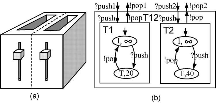
Two-slot toaster

Consider a toaster in which there are two slots that have their own start knobs as shown in Fig. 2(a). Each slot has the identical functionality except their toasting time. Initially, the knob is not pushed, but if one pushws the knob, the associated slot starts toasting for its toasting time: 20 seconds for the left slot, 40 seconds for the right slot. After the toasting time, each slot and its knobs pop up. Notice that even though one tries to push a knob when its associated slot is toasting, nothing happens.

One can model it with FD-DEVS as shown in Fig. 2(b). Two slots are modeled as atomic FD-DEVS whose input event is ``?push`` and output event is ``!pop``, states are ``Idle`` (I) and ``Toast`` (T) with the initial state is ``idle``. When it is ``Idle`` and receives ``?push`` (because one pushes the knob), its state changes to ``Toast``. In other words, it stays at ``Idle`` forever unless it receives ``?push`` event. 20 (res. 40) seconds later the left (res. right) slot returns to ``Idle``.

Formal Definition

where

The formal representation of the player in the ping-pong example shown in Fig. 1 can be given as follows. M =< X , Y , S , s 0 , τ , δ x , δ y > where X ={?receive}; Y ={!send}; S ={Send, Wait}; s 0 =Send for Player A, Wait for Player B; τ (Send)=0.1, τ (Wait)= ∞ ; δ x (Wait,?receive)=(Send,1), δ x (Send,?receive)=(Send,0); δ y (Send)=(!send, Wait), δ y (Wait)=( ϕ , Wait).

The formal representation of the slot of Two-slot Toaster Fig. 2(a) and (b) can be given as follows. M =< X , Y , S , s 0 , τ , δ x , δ y > where X ={?push}; Y ={!pop}; S ={I, T}; s 0 =I; τ (T)=20 for the left slot, 40 for the right slot, τ (I)= ∞ ; δ x (I, ?push)=(T,1), δ x (T,?push)=(T,0); δ y (T)=(!pop, I), δ y (I)=( ϕ , I).

As mentioned above, FD-DEVS is an relaxation of SP-DEVS. That means, FD-DEVS is a supper class of SP-DEVS. We would give a model of FD-DEVS of a crosswalk light controller which is used for SP-DEVS in this Wikipedia. M =< X , Y , S , s 0 , τ , δ x , δ y > where X ={?p}; Y ={!g:0, !g:1, !w:0, !w:1}; S ={BG, BW, G, GR, R, W, D}; s 0 =BG, τ (BG)=0.5, τ (BW)=0.5, τ (G)=30, τ (GR)=30, τ (R)=2, τ (W)=26, τ (D)=2; δ x (G,?p)=(GR,0), δ x (s,?p)=(s,0) if s ≠ G; δ y (BG)=(!g:1, BW), δ y (BW)=(!w:0, G), δ y (G)=( ϕ , G), δ y (GR)=(!g:0, R), δ y (R)=(!w:1, W), δ y (W)=(!w:0, D), δ y (D)=(!g:1, G);

Behaviors of FD-DEVS Models

A FD-DEVS model, M =< X , Y , S , s 0 , τ , δ x , δ y > is DEVS M =< X , Y , S ′ , s 0 ′ , t a , δ e x t , δ i n t , λ > where

δ e x t ( s , t s , t e , x ) = { ( s ′ , t s − t e ) if  δ x ( s , x ) = ( s ′ , 0 ) ( s ′ , τ ( s ′ ) ) if  δ x ( s , x ) = ( s ′ , 1 )

For details of DEVS behavior, the readers can refer to Behavior of Atomic DEVS

Fig. 3. shows an event segment (top) and the associated state trajectory (bottom) of Player A who plays the ping-pong game introduced in Fig. 1. In Fig. 3. the status of Player A is described as (state, lifespan, elapsed time)=( s , t s , t e ) and the line segment of the bottom of Fig. 3. denotes the value of the elapsed time. Since the initial state of Player A is ``Send`` and its lifetime is 0.1 seconds, the height of (Send, 0.1, t e ) is 0.1 which is the value of t s . After changing into (Wait, inf, 0) when t e is reset by 0, Player A doesn't know when t e becomes 0 again. However, since Player B sends back the ball to Player A 0.1 second later, Player A gets back to (Send, 0.1 0) at time 0.2. From that time, 0.1 seconds later when Player A's status becomes (Send, 0.1, 0.1), Player A sends back the ball to Player B and gets into (Wait, inf, 0). Thus, this cyclic state transitions which move ``Send`` to ``Wait`` back and forth will go forever.

Fig. 4. shows an event segment (top) and the associated state trajectory (bottom) of the left slot of the two-slot toaster introduced in Fig. 2. Like Fig.3, the status of the left slot is described as (state, lifespan, elapsed time)=( s , t s , t e ) in Fig. 4. Since the initial state of the toaster is ``I`` and its lifetime is infinity, the height of (Wait, inf, t e ) can be determined by when ?push occurs. Fig. 4. illustrates the case ?push happens at time 40 and the toaster changes into (T, 20, 0). From that time, 20 seconds later when its status becomes (T, 20, 20), the toaster gets back to (Wait, inf, 0) where we don't know when it gets back to ``Toast`` again. Fig. 4. shows the case that ?push occurs at time 90 so the toaster get into (T,20,0). Notice that even though there someone push again at time 97, that status (T, 20, 7) doesn't change at all because δ x (T,?push)=(T,1).

Applicability of Time-Zone Abstraction

The property of non-negative rational-valued lifespans which can be preserved or changed by input events along with finite numbers of states and events guarantees that the behavior of FD-DEVS networks can be abstracted as an equivalent finite-vertex reachability graph by abstracting the infinitely-many values of the elapsed times using the time abstracting technique introduced by Prof. D. Dill [Dill89]. An algorithm generating a finite-vertex reachability graph (RG)has been introduced in [HZ06a], [HZ07].

Reachability Graph

Fig. 5. shows the reachability graph of two-slot toaster which was shown in Fig. 2. In the reachability graph, each vertex has its own discrete state and time zone which are ranges of t e 1 , t e 2 and t e 1 − t e 2 . For example, for node (6) of Fig. 5, discrete state information is ((E, ∞ ),(T,40)), and time zone is 0 ≤ t e 1 ≤ 40 , 0 ≤ t e 2 ≤ 40 , − 20 ≤ t e 1 − t 21 ≤ 0 . Each directed arch shows how its source vertex changes into the destination vertex along with an associated event and a set of reset models. For example, the transition arc (6) to (5) is triggered by push1 event. At that time, the set {1} of the arc denotes that elapsed time of 1 (that is t e 1 is reset by 0 when transition (6) to (5) occurs. For more detailed information, the reader can refer to [HZ07].

Decidability of Safety

As a qualitative property, safety of a FD-DEVS network is decidable by (1) generating RG of the given network and (2) checking whether some bad states are reachable or not [HZ06b].

Decidability of Liveness

As a qualitative property, liveness of a FD-DEVS network is decidable by (1) generating RG of the given network, (2) from RG, generating kernel directed acyclic graph (KDAG) in which a vertex is strongly connected component, and (3) checking if a vertex of KDAG contains a state transition cycle which contains a set of liveness states[HZ06b].

Weak Expressiveness for describing nondeterminism

The features that all characteristic functions, τ , δ x , δ y of FD-DEVS are deterministic can be seen as somehow a limitation to model the system that has non-deterministic behaviors. For example, if a player of the ping-pong game shown in Fig. 1. has a stochastic lifespan at ``Send`` state, FD-DEVS doesn't capture the non-determinism effectively.

For Verification

There are two open source libraries DEVS# written in C# at http://xsy-csharp.sourceforge.net/DEVSsharp/ and XSY written in Python at https://code.google.com/p/x-s-y/ that support some reachability graph-based verification algorithms for finding safyness and liveness.

For Simulation via XML

For standardization of DEVS, especially using FDDEVS, Dr. Saurabh Mittal together with co-workers has worked on defining of XML format of FDDEVS. We can find an article at http://www.duniptechnologies.com/research/xfddevs/. This standard XML format was used for UML execution [RCMZ09] .