
 | ||
In decision theory and quantitative policy analysis, the expected value of including uncertainty (EVIU) is the expected difference in the value of a decision based on a probabilistic analysis versus a decision based on an analysis that ignores uncertainty.
Contents
Background
Decisions must be made every day in the ubiquitous presence of uncertainty. For most day-to-day decisions, various heuristics are used to act reasonably in the presence of uncertainty, often with little thought about its presence. However, for larger high-stakes decisions or decisions in highly public situations, decision makers may often benefit from a more systematic treatment of their decision problem, such as through quantitative analysis. To facilitate methodical analysis, while retaining transparency in the decision making process, analysts make use of quantitative modeling software such as Analytica. The academic field that focuses on this style of decision making and analysis is known as decision analysis.
When building a quantitative decision model, a model builder identifies various relevant factors, and encodes these as input variables. From these inputs, other quantities, called result variables, can be computed; these provide information for the decision maker. For example, in the example detailed below, I must decide how soon before my flight to leave for the airport (my decision). One input variable is how long it takes to drive from my house to the airport parking garage. From this and other inputs, the model can compute whether I'm likely to miss the flight and what the net cost (in minutes) will be for various decisions.
To reach a decision, a very common practice is to ignore uncertainty. Decisions are reached through quantitative analysis and model building by simply using a best guess (single value) for each input variable. Decisions are then made on computed point estimates. In many cases, however, ignoring uncertainty can lead to very poor decisions, with estimations for result variables often misleading the decision maker
An alternative to ignoring uncertainty in quantiative decision models is to explicitly encode uncertainty as part of the model. Due to the adoption of powerful software tools such as Analytica that allows representations of uncertainty to be explicitly encoded, along with high availability of computation power, this practice is becoming more commonplace among decision analytic modelers. With this approach, a probability distribution is provided for each input variable, rather than a single best guess. The variance in that distribution reflects the degree of subjective uncertainty (or lack of knowledge) in the input quantity. The software tools then use methods such as Monte Carlo analysis to propagate the uncertainty to result variables, so that a decision maker obtains an explicit picture of the impact that uncertainty has on his decisions, and in many cases can make a much better decision as a result.
When comparing the two approaches—ignoring uncertainty versus modeling uncertainty explicitly—the natural question to ask is how much difference it really makes to the quality of the decisions reached. In the 1960s, Ronald A. Howard proposed one such measure, the expected value of perfect information (EVPI), a measure of how much it would be worth to learn the "true" values for all uncertain input variables. While providing a highly useful measure of sensitivity to uncertainty, the EVPI does not directly capture the actual improvement in decisions obtained from explicitly representing and reasoning about uncertainty. For this, Max Henrion, in his Ph.D. thesis, introduced the expected value of including uncertainty (EVIU), the topic of this article.
Formalization
Let
When not including uncertainty, the optimal decision is found using only
The optimal decision taking uncertainty into account is the standard Bayes decision that maximizes expected utility:
The EVIU is the difference in expected utility between these two decisions:
The uncertain quantity x and decision variable d may each be composed of many scalar variables, in which case the spaces X and D are each vector spaces.
Example
The plane catching example described here is taken, with permission from Lumina Decision Systems, from an example model shipped with the Analytica visual modeling software.
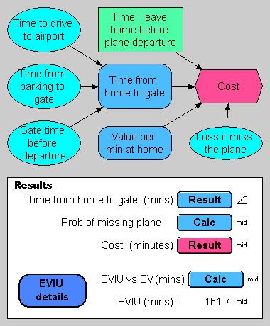
The diagram shows an influence diagram depiction of an Analytica model for deciding how early a person should leave home in order to catch a flight at the airport. The single decision, in the green rectangle, is the number of minutes that one will decide to leave prior to the plane's departure time. Four uncertain variables appear on the diagram in cyan ovals: The time required to drive from home to the airport's parking garage (in minutes), time to get from the parking garage to the gate (in minutes), the time before departure that one must be at the gate, and the loss (in minutes) incurred if the flight is missed. Each of these nodes contains a probability distribution, viz:
Time_to_drive_to_airport := LogNormal(median:60,gsdev:1.3)Time_from_parking_to_gate := LogNormal(median:10,gsdev:1.3)Gate_time_before_departure := Triangular(min:20,mode:30,max:40)Loss_if_miss_the_plane := LogNormal(median:400,stddev:100)Each of these distributions is taken to be statistically independent. The probability distribution for the first uncertain variable, Time_to_drive_to_airport, with median 60 and a geometric standard deviation of 1.3, is depicted in this graph:
The model calculates the cost (the red hexagonal variable) as the number of minutes (or minute equivalents) consumed to successfully board the plane. If one arrive too late, one will miss one's plane and incur the large loss (negative utility) of having to wait for the next flight. If one arrives too early, one incurs the cost of a needlessly long wait for the flight.
Models that utilize EVIU may use a utility function, or equivalently they may utilize a loss function, in which case the utility function is just the negative of the loss function. In either case, the EVIU will be positive. The main difference is just that with a loss function, the decision is made by minimizing loss rather than by maximizing utility. The example here uses a loss function, Cost.
The definitions for each of the computed variables is thus:
Time_from_home_to_gate := Time_to_drive_to_airport + Time_from_parking_to_gate + Loss_if_miss_the_planeValue_per_minute_at_home := 1Cost := Value_per_minute_at_home * Time_I_leave_home + (If Time_I_leave_home < Time_from_home_to_gate Then Loss_if_miss_the_plane Else 0)The following graph displays the expected value taking uncertainty into account (the smooth blue curve) to the expected utility ignoring uncertainty, graphed as a function of the decision variable.
When uncertainty is ignored, one acts as though the flight will be made with certainty as long as one leaves at least 100 minutes before the flight, and will miss the flight with certainty if one leaves any later than that. Because one acts as if everything is certain, the optimal action is to leave exactly 100 minutes (or 100 minutes, 1 second) before the flight.
When uncertainty is taken into account, the expected value smooths out (the blue curve), and the optimal action is to leave 140 minutes before the flight. The expected value curve, with a decision at 100 minutes before the flight, shows the expected cost when ignoring uncertainty to be 313.7 minutes, while the expected cost when one leaves 140 minute before the flight is 151 minutes. The difference between these two is the EVIU:
In other words, if uncertainty is explicitly taken into account when the decision is made, an average savings of 162.7 minutes will be realized.
Linear-quadratic control
In the context of centralized linear-quadratic control, with additive uncertainty in the equation of evolution but no uncertainty about coefficient values in that equation, the optimal solution for the control variables taking into account the uncertainty is the same as the solution ignoring uncertainty. This property, which gives a zero expected value of including uncertainty, is called certainty equivalence.
Relation to expected value of perfect information (EVPI)
Both EVIU and EVPI compare the expected value of the Bayes' decision with another decision made without uncertainty. For EVIU this other decision is made when the uncertainty is ignored, although it is there, while for EVPI this other decision is made after the uncertainty is removed by obtaining perfect information about x.
The EVPI is the expected cost of being uncertain about x, while the EVIU is the additional expected cost of assuming that one is certain.
The EVIU, like the EVPI, gives expected value in terms of the units of the utility function.