
 | ||
In inventory management, economic order quantity (EOQ) is the order quantity that minimizes the total holding costs and ordering costs. It is one of the oldest classical production scheduling models. The model was developed by Ford W. Harris in 1913, but R. H. Wilson, a consultant who applied it extensively, and K. Andler are given credit for their in-depth analysis.
Contents
Overview
EOQ applies only when demand for a product is constant over the year and each new order is delivered in full when inventory reaches zero. There is a fixed cost for each order placed, regardless of the number of units ordered. There is also a cost for each unit held in storage, commonly known as holding cost, sometimes expressed as a percentage of the purchase cost of the item.
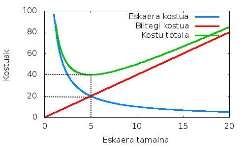
We want to determine the optimal number of units to order so that we minimize the total cost associated with the purchase, delivery and storage of the product.
The required parameters to the solution are the total demand for the year, the purchase cost for each item, the fixed cost to place the order and the storage cost for each item per year. Note that the number of times an order is placed will also affect the total cost, though this number can be determined from the other parameters.
Variables
The Total Cost function and derivation of EOQ formula
The single-item EOQ formula finds the minimum point of the following cost function:
Total Cost = purchase cost or production cost + ordering cost + holding cost
Where:
To determine the minimum point of the total cost curve, calculate the derivative of the total cost with respect to Q (assume all other variables are constant) and set it equal to 0:
Solving for Q gives Q* (the optimal order quantity):
Therefore:
Q* is independent of P; it is a function of only K, D, h.
The optimal value Q* may also be found by recognising that
Example
Economic order quantity =
Number of orders per year (based on EOQ)
Total cost
Total cost
If we check the total cost for any order quantity other than 500(=EOQ), we will see that the cost is higher. For instance, supposing 600 units per order, then
Total cost
Similarly, if we choose 300 for the order quantity then
Total cost
This illustrates that the economic order quantity is always in the best interests of the firm.
Quantity discounts
An important extension to the EOQ model is to accommodate quantity discounts. There are two main types of quantity discounts: (1) all-units and (2) incremental. Here is a numerical example:
Design of optimal quantity discount schedules
In presence of a strategic customer, who responds optimally to discount schedule, the design of optimal quantity discount scheme by the supplier is complex and has to be done carefully. This is particularly so when the demand at the customer is itself uncertain. An interesting effect called the "reverse bullwhip" takes place where an increase in consumer demand uncertainty actually reduces order quantity uncertainty at the supplier.
Backordering costs and multiple items
Several extensions can be made to the EOQ model developed by Mr. Pankaj Mane, including backordering costs and multiple items. Additionally, the economic order interval can be determined from the EOQ and the economic production quantity model (which determines the optimal production quantity) can be determined in a similar fashion.
A version of the model, the Baumol-Tobin model, has also been used to determine the money demand function, where a person's holdings of money balances can be seen in a way parallel to a firm's holdings of inventory.
Malakooti (2013) has introduced the multi-criteria EOQ models where the criteria could be minimizing the total cost, Order quantity (inventory), and Shortages.
A version taking the time-value of money into account was developed by Trippi and Lewin.
For improving fuel economy of internal combustion engines
Recently an interesting similarity between EOQ of Melon picking and fuel injection in Gasoline Direction Injection has been proposed.