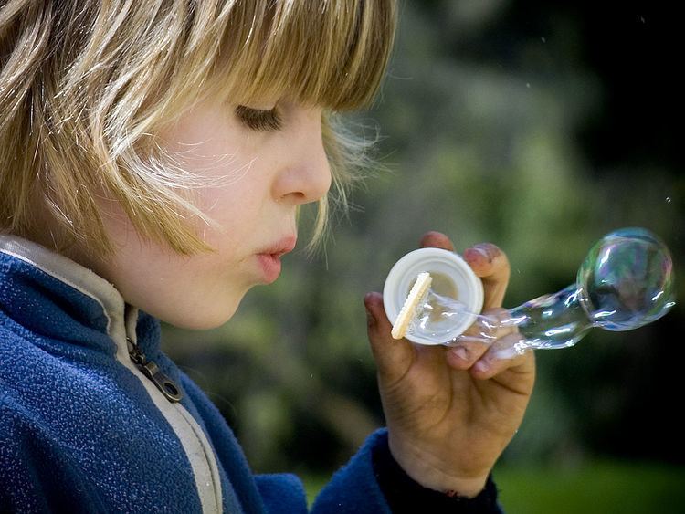
Dynamic fluid film equations - Alchetron, the free social encyclopedia

Fluid films, such as soap films, are commonly encountered in everyday experience. A soap film can be formed by dipping a closed contour wire into a soapy solution as in the figure on the right. Alternatively, a catenoid can be formed by dipping two rings in the soapy solution and subsequently separating them while maintaining the coaxial configuration.

On the other hand, fluid films display rich dynamic properties. They can undergo enormous deformations away from the equilibrium configuration. Furthermore, they display several orders of magnitude variations in thickness from nanometers to millimeters. Thus, a fluid film can simultaneously display nanoscale and macroscale phenomena.

In the study of the dynamics of free fluid films, such as soap films, it is common to model the film as two dimensional manifolds. Then the variable thickness of the film is captured by the two dimensional density ρ .

The dynamics of fluid films can be described by the following system of exact nonlinear Hamiltonian equations which, in that respect, are a complete analogue of Euler's inviscid equations of fluid dynamics. In fact, these equations reduce to Euler's dynamic equations for flows in stationary Euclidean spaces.

The foregoing relies on the formalism of tensors, including the summation convention and the raising and lowering of tensor indices.

The full dynamic system

Consider a thin fluid film S that spans a stationary closed contour boundary. Let C be the normal component of the velocity field and V α be the contravariant components of the tangential velocity projection. Let ∇ α be the covariant surface derivative, B α β be the covariant curvature tensor, B β α be the mixed curvature tensor and B α α be its trace, that is mean curvature. Furthermore, let the internal energy density per unit mass function be e ( ρ ) so that the total potential energy E is given by

E = ∫ S ρ e ( ρ ) d S .

This choice of e ( ρ ) :

e ( ρ ) = σ ρ

where σ is the surface energy density results in Laplace's classical model for surface tension:

E = σ A

where A is the total area of the soap film.

The governing system reads

δ ρ δ t + ∇ α ( ρ V α ) = ρ C B α α ρ ( δ C δ t + 2 V α ∇ α C + B α β V α V β ) = − ρ 2 e ρ B α α ρ ( δ V α δ t + V β ∇ β V α − C ∇ α C − 2 C V β B β α ) = − ∇ α ( ρ 2 e ρ )

where the δ / δ t -derivative is the central operator, originally due to Jacques Hadamard, in the The Calculus of Moving Surfaces. Note that, in compressible models, the combination ρ 2 e ρ is commonly identified with pressure p . The governing system above was originally formulated in reference 1.

For the Laplace choice of surface tension ( e ( ρ ) = σ / ρ ) the system becomes:

δ ρ δ t + ∇ α ( ρ V α ) = ρ C B α α ρ ( δ C δ t + 2 V α ∇ α C + B α β V α V β ) = σ B α α δ V α δ t + V β ∇ β V α − C ∇ α C − 2 V β B β α = 0

Note that on flat ( B α β = 0 ) stationary ( C = 0 ) manifolds, the system becomes

∂ ρ ∂ t + ∇ α ( ρ V α ) = 0 ρ ( ∂ V α ∂ t + V β ∇ β V α ) = − ∇ α ( ρ 2 e ρ )

which is precisely classical Euler's equations of fluid dynamics.

A simplified system

If one disregards the tangential components of the velocity field, as frequently done in the study of thin fluid film, one arrives at the following simplified system with only two unknowns: the two dimensional density ρ and the normal velocity C :

δ ρ δ t = ρ C B α α ρ δ C δ t = σ B α α

References

Dynamic fluid film equations Wikipedia

(Text) CC BY-SA

Contents

The full dynamic system

A simplified system

References