The Duffing equation (or Duffing oscillator), named after Georg Duffing (1861–1944), is a non-linear second-order differential equation used to model certain damped and driven oscillators. The equation is given by
x
¨
+
δ
x
˙
+
α
x
+
β
x
3
=
γ
cos
(
ω
t
)
where the (unknown) function
x
=
x
(
t
)
is the displacement at time
t
,
x
˙
is the first derivative of
x
with respect to time, i.e. velocity, and
x
¨
is the second time-derivative of
x
,
i.e. acceleration. The numbers
δ
,
α
,
β
,
γ
and
ω
are given constants.
The equation describes the motion of a damped oscillator with a more complex potential than in simple harmonic motion (which corresponds to the case
β
=
δ
=
0
); in physical terms, it models, for example, a spring pendulum whose spring's stiffness does not exactly obey Hooke's law.
The Duffing equation is an example of a dynamical system that exhibits chaotic behavior. Moreover, the Duffing system presents in the frequency response the jump resonance phenomenon that is a sort of frequency hysteresis behaviour.
The parameters in the above equation are:
δ
controls the amount of damping,
α
controls the linear stiffness,
β
controls the amount of non-linearity in the restoring force; if
β
=
0
,
the Duffing equation describes a damped and driven simple harmonic oscillator,
γ
is the amplitude of the periodic driving force; if
γ
=
0
the system is without a driving force, and
ω
is the angular frequency of the periodic driving force.
The Duffing equation can be seen as describing the oscillations of a mass attached to a nonlinear spring and a linear damper. The restoring force provided by the nonlinear spring is then
α
x
+
β
x
3
.
When
α
>
0
and
β
>
0
the spring is called a hardening spring. Conversely, for
β
<
0
it is a softening spring (still with
α
>
0
). Consequently, the adjectives hardening and softening are used with respect to the Duffing equation in general, dependent on the values of
β
(and
α
).
The number of parameters in the Duffing equation can be reduced by two through scaling, e.g. the excursion
x
and time
t
can be scaled as:
τ
=
t
α
and
y
=
x
α
/
γ
,
assuming
α
is positive (other scalings are possible for different ranges of the parameters, or for different emphasis in the problem studied). Then:
y
¨
+
2
η
y
˙
+
y
+
ε
y
3
=
cos
(
σ
τ
)
,
where
η
=
δ
2
α
,
ε
=
β
γ
2
α
3
.
and
σ
=
ω
α
.
The dots denote differentiation of
y
(
τ
)
with respect to
τ
.
This shows that the solutions to the forced and damped Duffing equation can be described in terms of the three parameters (
ε
,
η
and
σ
) and two initial conditions (i.e. for
y
(
t
0
)
and
y
˙
(
t
0
)
).
In general, the Duffing equation does not admit an exact symbolic solution. However, many approximate methods work well:
Expansion in a Fourier series may provide an equation of motion to arbitrary precision.
The
x
3
term, also called the Duffing term, can be approximated as small and the system treated as a perturbed simple harmonic oscillator.
The Frobenius method yields a complex but workable solution.
Any of the various numeric methods such as Euler's method and Runge-Kutta can be used.
The homotopy analysis method (HAM) has also been reported for obtaining approximate solutions of the Duffing equation, also for strong nonlinearity.
In the special case of the undamped (
δ
=
0
) and undriven (
γ
=
0
) Duffing equation, an exact solution can be obtained using Jacobi's elliptic functions.
Multiplication of the undamped and unforced Duffing equation,
γ
=
δ
=
0
,
with
x
˙
gives:
x
˙
(
x
¨
+
α
x
+
β
x
3
)
=
0
⇒
d
d
t
[
1
2
(
x
˙
)
2
+
1
2
α
x
2
+
1
4
β
x
4
]
=
0
⇒
1
2
(
x
˙
)
2
+
1
2
α
x
2
+
1
4
β
x
4
=
H
,
with H a constant. The value of H is determined by the initial conditions
x
(
0
)
and
x
˙
(
0
)
.
The substitution
y
=
x
˙
in H shows that the system is Hamiltonian:
x
˙
=
+
∂
H
∂
y
,
y
˙
=
−
∂
H
∂
x
with
H
=
1
2
y
2
+
1
2
α
x
2
+
1
4
β
x
4
.
When both
α
and
β
are positive, the solution is bounded:
|
x
|
≤
2
H
/
α
and
|
x
˙
|
≤
2
H
,
with the Hamiltonian H being positive.
Similarly, for the damped oscillator,
x
˙
(
x
¨
+
δ
x
˙
+
α
x
+
β
x
3
)
=
0
⇒
d
d
t
[
1
2
(
x
˙
)
2
+
1
2
α
x
2
+
1
4
β
x
4
]
=
−
δ
(
x
˙
)
2
⇒
d
H
d
t
=
−
δ
(
x
˙
)
2
≤
0
,
since
δ
≥
0
for damping. Without forcing the damped Duffing oscillator will end up at (one of) its stable equilibrium point(s). The equilibrium points, stable and unstable, are at
α
x
+
β
x
3
=
0.
If
α
>
0
the stable equilibrium is at
x
=
0.
If
α
<
0
and
β
>
0
the stable equilibria are at
x
=
+
−
α
/
β
and
x
=
−
−
α
/
β
.
The forced Duffing oscillator with cubic nonlinearity is described by the following ordinary differential equation:
x
¨
+
δ
x
˙
+
α
x
+
β
x
3
=
γ
cos
(
ω
t
)
.
The frequency response of this oscillator describes the amplitude
z
of steady state response of the equation (i.e.
x
(
t
)
) at a given frequency of excitation
ω
.
For a linear oscillator with
β
=
0
,
the frequency response is also linear. However, for a nonzero cubic coefficient, the frequency response becomes nonlinear. Depending on the type of nonlinearity, the Duffing oscillator can show hardening, softening or mixed hardening–softening frequency response. Anyway, using the homotopy analysis method or harmonic balance, one can derive a frequency response equation in the following form:
[
(
ω
2
−
α
−
3
4
β
z
2
)
2
+
(
δ
ω
)
2
]
z
2
=
γ
2
.
For the parameters of the Duffing equation, the above algebraic equation gives the steady state oscillation amplitude
z
at a given excitation frequency.
For certain ranges of the parameters in the Duffing equation, the frequency response may no longer be a single-valued function of forcing frequency
ω
.
For a hardening spring oscillator (
α
>
0
and large enough positive
β
>
β
c
+
>
0
) the frequency response overhangs to the high-frequency side, and to the low-frequency side for the softening spring oscillator (
α
>
0
and
β
<
β
c
−
<
0
). The lower overhanging side is unstable – i.e. the dashed-line parts in the figures of the frequency response – and cannot be realized for a sustained time. Consequently, the jump phenomenon shows up:
when the angular frequency
ω
is slowly increased (with other parameters fixed), the response amplitude
z
drops at A suddenly to B,
if the frequency
ω
is slowly decreased, then at C the amplitude jumps up to D, thereafter following the upper branch of the frequency response.
The jumps A–B and C–D do not coincide, but the system shows hysteresis depending on the frequency sweep direction.
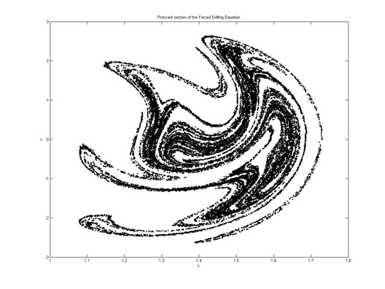
Some typical examples of the time series and phase portraits of the Duffing equation, showing the appearance of subharmonics through period-doubling bifurcation – as well chaotic behavior – are shown in the figures below. The forcing amplitude increases from
γ
=
0.20
to
γ
=
0.65.
The other parameters have the values:
α
=
−
1
,
β
=
+
1
,
δ
=
0.3
and
ω
=
1.2.
The initial conditions are
x
(
0
)
=
1
and
x
˙
(
0
)
=
0.
The red dots in the phase portraits are at times
t
which are an integer multiple of the period
T
=
2
π
/
ω
.