Dual curve

Equations

Let f(x, y, z)=0 be the equation of a curve in homogeneous coordinates. Let Xx+Yy+Zz=0 be the equation of a line, with (X, Y, Z) being designated its line coordinates. The condition that the line is tangent to the curve can be expressed in the form F(X, Y, Z)=0 which is the tangential equation of the curve.

Let (p, q, r) be the point on the curve, then the equation of the tangent at this point is given by

So Xx+Yy+Zz=0 is a tangent to the curve if

Eliminating p, q, r, and λ from these equations, along with Xp+Yq+Zr=0, gives the equation in X, Y and Z of the dual curve.

For example, let C be the conic ax²+by²+cz²=0. Then dual is found by eliminating p, q, r, and λ from the equations

The first three equations are easily solved for p, q, r, and substituting in the last equation produces

Clearing 2λ from the denominators, the equation of the dual is

For a parametrically defined curve its dual curve is defined by the following parametric equations:

The dual of an inflection point will give a cusp and two points sharing the same tangent line will give a self intersection point on the dual.

Degree

If X is a plane algebraic curve then the degree of the dual is the number of points intersection with a line in the dual plane. Since a line in the dual plane corresponds to a point in the plane, the degree of the dual is the number of tangents to the X that can be drawn through a given point. The points where these tangents touch the curve are the points of intersection between the curve and the polar curve with respect to the given point. If the degree of the curve is d then the degree of the polar is d−1 and so the number of tangents that can be drawn through the given point is at most d(d−1).

The dual of a line (a curve of degree 1) is an exception to this and is taken to be a point in the dual space (namely the original line). The dual of a single point is taken to be the collection of lines though the point; this forms a line in the dual space which corresponds to the original point.

If X is smooth, i.e. there are no singular points then the dual of X has the maximum degree d(d − 1). If X is a conic this implies its dual is also a conic. This can also be seen geometrically: the map from a conic to its dual is 1-to-1 (since no line is tangent to two points of a conic, as that requires degree 4), and tangent line varies smoothly (as the curve is convex, so the slope of the tangent line changes monotonically: cusps in the dual require an inflection point in the original curve, which requires degree 3).

For curves with singular points, these points will also lie on the intersection of the curve and its polar and this reduces the number of possible tangent lines. The degree of the dual given in terms of the d and the number and types of singular points of X is one of the Plücker formulas.

Polar reciprocal

The dual can be visualized as a locus in the plane in the form of the polar reciprocal. This is defined with reference to a fixed conic Q as the locus of the poles of the tangent lines of the curve C. The conic Q is nearly always taken to be a circle and this case the polar reciprocal is the inverse of the pedal of C.

Properties of dual curve

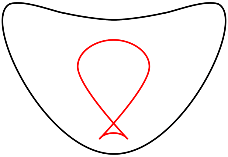
Properties of the original curve correspond to dual properties on the dual curve. In the image at right, the red curve has three singularities – a node in the center, and two cusps at the lower right and lower left. The black curve has no singularities, but has four distinguished points: the two top-most points have the same tangent line (a horizontal line), while there are two inflection points on the upper curve. The two top-most points correspond to the node (double point), as they both have the same tangent line, hence map to the same point in the dual curve, while the inflection points correspond to the cusps, corresponding to the tangent lines first going one way, then the other (slope increasing, then decreasing).

By contrast, on a smooth, convex curve the angle of the tangent line changes monotonically, and the resulting dual curve is also smooth and convex.

Further, both curves have a reflectional symmetry, corresponding to the fact that symmetries of a projective space correspond to symmetries of the dual space, and that duality of curves is preserved by this, so dual curves have the same symmetry group. In this case both symmetries are realized as a left-right reflection; this is an artifact of how the space and the dual space have been identified – in general these are symmetries of different spaces.

Higher dimensions

Similarly, generalizing to higher dimensions, given a hypersurface, the tangent space at each point gives a family of hyperplanes, and thus defines a dual hypersurface in the dual space. For any closed subvariety X in a projective space, the set of all hyperplanes tangent to some point of X is a closed subvariety of the dual of the projective projective, called the dual variety of X.

Examples

Dual polygon

The dual curve construction works even if the curve is piecewise linear (or piecewise differentiable, but the resulting map is degenerate (if there are linear components) or ill-defined (if there are singular points).

In the case of a polygon, all points on each edge share the same tangent line, and thus map to the same vertex of the dual, while the tangent line of a vertex is ill-defined, and can be interpreted as all the lines passing through it with angle between the two edges. This accords both with projective duality (lines map to points, and points to lines), and with the limit of smooth curves with no linear component: as a curve flattens to an edge, its tangent lines map to closer and closer points; as a curve sharpens to a vertex, its tangent lines spread further apart.