Distributive lattice

Definition

As in the case of arbitrary lattices, one can choose to consider a distributive lattice L either as a structure of order theory or of universal algebra. Both views and their mutual correspondence are discussed in the article on lattices. In the present situation, the algebraic description appears to be more convenient:

A lattice (L,∨,∧) is distributive if the following additional identity holds for all x, y, and z in L:

x ∧ (y ∨ z) = (x ∧ y) ∨ (x ∧ z).

Viewing lattices as partially ordered sets, this says that the meet operation preserves non-empty finite joins. It is a basic fact of lattice theory that the above condition is equivalent to its dual:

x ∨ (y ∧ z) = (x ∨ y) ∧ (x ∨ z)   for all x, y, and z in L.

In every lattice, defining p≤q as usual to mean p∧q=p, the inequality x ∧ (y ∨ z) ≥ (x ∧ y) ∨ (x ∧ z) holds as well as its dual inequality x ∨ (y ∧ z) ≤ (x ∨ y) ∧ (x ∨ z). A lattice is distributive if one of the converse inequalities holds, too. More information on the relationship of this condition to other distributivity conditions of order theory can be found in the article on distributivity (order theory).

Morphisms

A morphism of distributive lattices is just a lattice homomorphism as given in the article on lattices, i.e. a function that is compatible with the two lattice operations. Because such a morphism of lattices preserves the lattice structure, it will consequently also preserve the distributivity (and thus be a morphism of distributive lattices).

Examples

Distributive lattices are ubiquitous but also rather specific structures. As already mentioned the main example for distributive lattices are lattices of sets, where join and meet are given by the usual set-theoretic operations. Further examples include:

The Lindenbaum algebra of most logics that support conjunction and disjunction is a distributive lattice, i.e. "and" distributes over "or" and vice versa.

Every Boolean algebra is a distributive lattice.

Every Heyting algebra is a distributive lattice. Especially this includes all locales and hence all open set lattices of topological spaces. Also note that Heyting algebras can be viewed as Lindenbaum algebras of intuitionistic logic, which makes them a special case of the above example.

Every totally ordered set is a distributive lattice with max as join and min as meet.

The natural numbers form a (conditionally complete) distributive lattice by taking the greatest common divisor as meet and the least common multiple as join. This lattice also has a least element, namely 1, which therefore serves as the identity element for joins.

Given a positive integer n, the set of all positive divisors of n forms a distributive lattice, again with the greatest common divisor as meet and the least common multiple as join. This is a Boolean algebra if and only if n is square-free.

A lattice-ordered vector space is a distributive lattice.

Young's lattice given by the inclusion ordering of Young diagrams representing integer partitions is a distributive lattice.

Early in the development of the lattice theory Charles S. Peirce believed that all lattices are distributive, that is, distributivity follows from the rest of the lattice axioms. However, independence proofs were given by Schröder, Voigt,^(de) Lüroth, Korselt, and Dedekind.

Characteristic properties

Various equivalent formulations to the above definition exist. For example, L is distributive if and only if the following holds for all elements x, y, z in L:

(x ∧ y) ∨ (y ∧ z) ∨ (z ∧ x) = (x ∨ y) ∧ (y ∨ z) ∧ (z ∨ x).

Similarly, L is distributive if and only if

x ∧ z = y ∧ z and x ∨ z = y ∨ z always imply x=y.

Hasse diagrams of the two prototypical non-distributive lattices

The simplest non-distributive lattices are M₃, the "diamond lattice", and N₅, the "pentagon lattice". A lattice is distributive if and only if none of its sublattices is isomorphic to M₃ or N₅; a sublattice is a subset that is closed under the meet and join operations of the original lattice. Note that this is not the same as being a subset that is a lattice under the original order (but possibly with different join and meet operations). Further characterizations derive from the representation theory in the next section.

Finally distributivity entails several other pleasant properties. For example, an element of a distributive lattice is meet-prime if and only if it is meet-irreducible, though the latter is in general a weaker property. By duality, the same is true for join-prime and join-irreducible elements. If a lattice is distributive, its covering relation forms a median graph.

Furthermore, every distributive lattice is also modular.

Representation theory

The introduction already hinted at the most important characterization for distributive lattices: a lattice is distributive if and only if it is isomorphic to a lattice of sets (closed under set union and intersection). That set union and intersection are indeed distributive in the above sense is an elementary fact. The other direction is less trivial, in that it requires the representation theorems stated below. The important insight from this characterization is that the identities (equations) that hold in all distributive lattices are exactly the ones that hold in all lattices of sets in the above sense.

Birkhoff's representation theorem for distributive lattices states that every finite distributive lattice is isomorphic to the lattice of lower sets of the poset of its join-prime (equivalently: join-irreducible) elements. This establishes a bijection (up to isomorphism) between the class of all finite posets and the class of all finite distributive lattices. This bijection can be extended to a duality of categories between homomorphisms of finite distributive lattices and monotone functions of finite posets. Generalizing this result to infinite lattices, however, requires adding further structure.

Another early representation theorem is now known as Stone's representation theorem for distributive lattices (the name honors Marshall Harvey Stone, who first proved it). It characterizes distributive lattices as the lattices of compact open sets of certain topological spaces. This result can be viewed both as a generalization of Stone's famous representation theorem for Boolean algebras and as a specialization of the general setting of Stone duality.

A further important representation was established by Hilary Priestley in her representation theorem for distributive lattices. In this formulation, a distributive lattice is used to construct a topological space with an additional partial order on its points, yielding a (completely order-separated) ordered Stone space (or Priestley space). The original lattice is recovered as the collection of clopen lower sets of this space.

As a consequence of Stone's and Priestley's theorems, one easily sees that any distributive lattice is really isomorphic to a lattice of sets. However, the proofs of both statements require the Boolean prime ideal theorem, a weak form of the axiom of choice.

Free distributive lattices

The free distributive lattice over a set of generators G can be constructed much more easily than a general free lattice. The first observation is that, using the laws of distributivity, every term formed by the binary operations ∨ and ∧ on a set of generators can be transformed into the following equivalent normal form:

M₁ ∨ M₂ ∨ ... ∨ M_n

where the M_i are finite meets of elements of G. Moreover, since both meet and join are commutative and idempotent, one can ignore duplicates and order, and represent a join of meets like the one above as a set of sets:

{N₁, N₂, ..., N_n},

where the N_i are finite subsets of G. However, it is still possible that two such terms denote the same element of the distributive lattice. This occurs when there are indices j and k such that N_j is a subset of N_k. In this case the meet of N_k will be below the meet of N_j, and hence one can safely remove the redundant set N_k without changing the interpretation of the whole term. Consequently, a set of finite subsets of G will be called irredundant whenever all of its elements N_i are mutually incomparable (with respect to the subset ordering); that is, when it forms an antichain of finite sets.

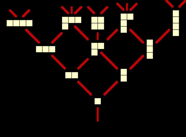
Now the free distributive lattice over a set of generators G is defined on the set of all finite irredundant sets of finite subsets of G. The join of two finite irredundant sets is obtained from their union by removing all redundant sets. Likewise the meet of two sets S and T is the irredundant version of { N ∪ M | N in S, M in T}. The verification that this structure is a distributive lattice with the required universal property is routine.

The number of elements in free distributive lattices with n generators is given by the Dedekind numbers. These numbers grow rapidly, and are known only for n ≤ 8; they are

2, 3, 6, 20, 168, 7581, 7828354, 2414682040998, 56130437228687557907788 (sequence A000372 in the OEIS).

The numbers above count the number of free distributive lattices in which the lattice operations are joins and meets of finite sets of elements, including the empty set. If empty joins and empty meets are disallowed, the resulting free distributive lattices have two fewer elements; their numbers of elements form the sequence

1, 4, 18, 166, 7579, 7828352, 2414682040996, 56130437228687557907786 (sequence A007153 in the OEIS).