Debye–Hückel equation

Debye–Hückel limiting law

For the principles used to derive this equation see Debye–Hückel theory

In order to calculate the activity,   a C , of an ion, C, in a solution, one must know the concentration and the activity coefficient:

  a C = γ [ C ] [ C ⊖ ]

where

  γ is the activity coefficient of C   [ C ⊖ ] is the concentration of the chosen standard state, e.g. 1 mol/kg if we work in molality. [ C ] is a measure of the concentration of C Dividing [ C ] with [ C ⊖ ] gives a dimensionless quantity

The Debye–Hückel limiting law enables one to determine the activity coefficient of an ion in a dilute solution of known ionic strength. The equation is^[1]

ln ⁡ ( γ i ) = − z i 2 q 2 κ 8 π ε r ε 0 k B T = − z i 2 q 3 N A 1 / 2 4 π ( ε r ε 0 k B T ) 3 / 2 I 2 = − A z i 2 I z i is the charge number of ion species i q is the elementary charge κ is the inverse of the Debye screening length, defined below ε r is the relative permittivity of the solvent ε 0 is the permittivity of free space k B is Boltzmann's constant T is the temperature of the solution N A is Avogadro's number I is the ionic strength of the solution, defined below A is a constant that depends on temperature. If I is expressed in terms of molality, instead of molarity (as in the equation above and in the rest of this article), then an experimental value for A of water is 1.172  mol − 1 / 2  kg 1 / 2 at 25 C. It is common to use a base-10 logarithm, in which case we factor ln ⁡ 10 , so A is 0.509  mol − 1 / 2  kg 1 / 2 .

It is important to note that because the ions in the solution act together, the activity coefficient obtained from this equation is actually a mean activity coefficient.

The excess osmotic pressure which is obtained from Debye–Hückel theory is in cgs units:

P e x = − k B T κ c g s 3 24 π = − k B T ( 4 π ∑ j c j q j ϵ 0 ϵ r k B T ) 3 / 2 24 π .

Therefore the total pressure is the sum of the excess osmotic pressure and the ideal pressure P i d = k B T ∑ i c i . The osmotic coefficient is then given by:

ϕ = P i d + P e x P i d = 1 + P e x P i d

Summary of Debye and Hückel's first paper on the theory of dilute electrolytes

The English title of the paper is called "On the Theory of Electrolytes. I. Freezing Point Depression and Related Phenomena." It was originally published in volume 24 of a German-language journal, called Physikalische Zeitschrift, in 1923. An English translationof the paper is included in a book of collected papers presented to Debye by "his pupils, friends, and the publishers on the occasion of his seventieth birthday on March 24, 1954." The paper deals with the calculation of properties of electrolyte solutions that are not under the influence of net electric fields, thus it deals with electrostatics.

In the same year they first published this paper, Debye and Hückel, hereinafter D&H, also released a paper that covered their initial characterization of solutions under the influence of electric fields called "On the Theory of Electrolytes. II. Limiting Law for Electric Conductivity," but that subsequent paper is not (yet) covered here.

In the following summary (as yet incomplete and unchecked), modern notation and terminology are used, from both chemistry and mathematics, in order to prevent confusion. Also, with a few exceptions to improve clarity, the subsections in this summary are (very) condensed versions of the same subsections of the original paper.

Introduction

D&H note that the Guldberg–Waage formula for electrolyte species in chemical reaction equilibrium in classical form is

∏ i = 1 s x i ν i = K

D&H say that, due to the "mutual electrostatic forces between the ions," it is necessary to modify the Guldberg–Waage equation by replacing K with γ K , where γ is an overall activity coefficient, not a "special" activity coefficient (a separate activity coefficient associated with each species)—which is what is used in modern chemistry as of 2007.

The relationship between γ and the special activity coefficients, γ i is

log ⁡ ( γ ) = ∑ i = 1 s ν i log ⁡ ( γ i ) .

Fundamentals

D&H use the Helmholtz and Gibbs free entropies, Φ and Ξ , to express the effect of electrostatic forces in an electrolyte on its thermodynamic state. Specifically, they split most of the thermodynamic potentials into classical and electrostatic terms.

Φ = S − U T = − A T

D&H give the total differential of Φ as

d Φ = P T d V + U T 2 d T

By the definition of the total differential, this means that

which are useful further on.

As stated previously, the internal energy is divided into two parts,

U = U k + U e

Similarly, the Helmholtz free entropy is also divided into two parts,

Φ = Φ k + Φ e

D&H state, without giving the logic, that

Φ e = ∫ U e T 2 d T

It would seem that, without some justification,

Φ e = ∫ P e T d V + ∫ U e T 2 d T .

Without mentioning it specifically, D&H later give what might be the required (above) justification while arguing that Φ e = Ξ e , an assumption that the solvent is incompressible.

The definition of the Gibbs free entropy, Ξ , is

Ξ = S − U + P V T = Φ − P V T = − G T .

D&H give the total differential of Ξ as

d Ξ = − V T d P + U + P V T 2 d T .

At this point D&H note that, for water containing 1 mole per liter of potassium chloride (nominal pressure and temperature aren't given), the electric pressure, P e , amounts to 20 atmospheres. Furthermore, they note that this level of pressure gives a relative volume change of 0.001. Therefore, they neglect change in volume of water due to electric pressure, writing

Ξ = Ξ k + Ξ e

and put

Ξ e = Φ e = ∫ U e T 2 d T .

D&H say that, according to Planck, the classical part of the Gibbs free entropy is

Ξ k = ∑ i = 0 s N i ( ξ i − k B l n ( x i ) ) . i is a species s is the number of different particle types in solution N i is the number of particles of species i ξ i is the particle specific Gibbs free entropy of species i k B is Boltzmann's constant x i is the mole fraction of species i

Species zero is the solvent. The definition of ξ i is as follows, where lower case letters indicate the particle specific versions of the corresponding extensive properties:

ξ i = s i − u i + P v i T .

D&H don't say so, but the functional form for Ξ k may be derived from the functional dependence of the chemical potential of a component of an ideal mixture upon its mole fraction.

D&H note that the internal energy, U , of a solution is lowered by the electrical interaction of its ions, but that this effect can't be determined by using the crystallographic approximation for distances between dissimilar atoms (the cube root of the ratio of total volume to the number of particles in the volume). This is because there is more thermal motion in a liquid solution than in a crystal. The thermal motion tends to smear out the natural lattice that would otherwise be constructed by the ions. Instead, D&H introduce the concept of an ionic atmosphere or cloud. Like the crystal lattice, each ion still attempts to surround itself with oppositely charged ions, but in a more free-form manner; at small distances away from positive ions, one is more likely to find negative ions and vice versa.

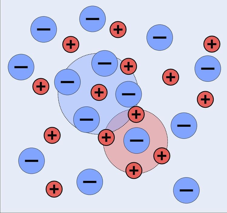
The potential energy of an arbitrary ion solution

Electroneutrality of a solution requires that

∑ i = 1 s N i z i = 0. N i is the total number of ions of species i in the solution z i is the charge number of species i.

To bring an ion of species i, initially far away, to a point P within the ion cloud requires interaction energy in the amount of z i q φ , where q is the elementary charge and φ is the value of the scalar electric potential field at P . If electric forces were the only factor in play, the minimum energy configuration of all the ions would be achieved in a close-packed lattice configuration. However, the ions are in thermal equilibrium with each other and they are relatively free to move. Thus they obey Boltzmann statistics and form a Boltzmann distribution. All species' number densities, n i , are altered from their bulk (overall average) values, n i 0 , by the corresponding Boltzmann factor, e − z i q φ k B T , where k B is the Boltzmann constant and T is the temperature (http://www.pma.caltech.edu/Courses/ph136/yr2006/text.html, section 19.3). Thus,

n i = N i V e − z i q φ k B T = n i 0 e − z i q φ k B T V is the volume of the solution

at every point in the cloud. Note that in the infinite temperature limit, all ions are distributed uniformly, with no regard for their electrostatic interactions.

The charge density is related to the number density:

ρ = ∑ i z i q n i = ∑ i z i q n i 0 e − z i q φ k B T .

When combining this result for the charge density with the Poisson equation from electrostatics, a form of the Poisson–Boltzmann equation results:

∇ 2 φ = − ρ ε r ε 0 = − ∑ i z i q n i 0 ε r ε 0 e − z i q φ k B T .

This equation is difficult to solve and does not follow the principle of linear superposition for the relationship between the number of charges and the strength of the potential field. It has been solved by the Swedish mathematician Thomas Hakon Gronwall and his collaborators physicical chemists V.K. La Mer and Karl Sandved in a 1928 paper from Physikalische Zeitschrift which deals with extensions to Debye-Huckel theory which resorted to Taylor series expansion.

However, for sufficiently low concentrations of ions, a first order Taylor series expansion approximation for the exponential function may be used ( e x = 1 + x for 0 < x ≪ 1 ) to create a linear differential equation (Hamann, Hamnett, and Vielstich. Electrochemistry. Wiley-VCH. section 2.4.2). D&H say that this approximation holds at large distances between ions, which is the same as saying that the concentration is low. Lastly, they claim without proof that the addition of more terms in the expansion has little effect on the final solution. Thus,

− ∑ i z i q n i 0 ε r ε 0 e − z i q φ k B T ≈ − ∑ i z i q n i 0 ε r ε 0 ( 1 − z i q φ k B T ) = − ( ∑ i z i q n i 0 ε r ε 0 − ∑ i z i 2 q 2 n i 0 φ ε r ε 0 k B T ) .

The Poisson–Boltzmann equation is transformed to

∇ 2 φ = ∑ i z i 2 q 2 n i 0 φ ε r ε 0 k B T ,

because the first summation is zero due to electroneutrality.

Factor out the scalar potential and assign the leftovers, which are constant, to κ 2 . Also, let I be the ionic strength of the solution:

κ 2 = ∑ i z i 2 q 2 n i 0 ε r ε 0 k B T = 2 I q 2 ε r ε 0 k B T , I = 1 2 ∑ i z i 2 n i 0 .

So, the fundamental equation is reduced to a form of the Helmholtz equation:(http://guava.physics.uiuc.edu/~nigel/courses/569/Essays_2004/files/lu.pdf section 3.1)

∇ 2 φ = κ 2 φ .

Today, κ − 1 is called the Debye screening length. D&H recognize the importance of the parameter in their paper and characterize it as a measure of the thickness of the ion atmosphere, which is an electrical double layer of the Guoy–Chapman type.

The equation may be expressed in spherical coordinates by taking r = 0 at some arbitrary ion (http://hyperphysics.phy-astr.gsu.edu/hbase/electric/laplace.html):

∇ 2 φ = 1 r 2 ∂ ∂ r ( r 2 ∂ φ ( r ) ∂ r ) = ∂ 2 φ ( r ) ∂ r 2 + 2 r ∂ φ ( r ) ∂ r = κ 2 φ ( r ) .

The equation has the following general solution; keep in mind that κ is a positive constant:

φ ( r ) = A e − κ 2 r r + A ′ e κ 2 r 2 r κ 2 = A e − κ r r + A ″ e κ r r = A e − κ r r . A , A ′ , and A ″ are undetermined constants

The electric potential is zero at infinity by definition, so A ″ must be zero.

In the next step, D&H assume that there is a certain radius, a i , beyond which no ions in the atmosphere may approach the (charge) center of the singled out ion. This radius may be due to the physical size of the ion itself, the sizes of the ions in the cloud, and any water molecules that surround the ions. Mathematically, they treat the singled out ion as a point charge to which one may not approach within the radius a i .

The potential of a point charge by itself is:

φ p c ( r ) = 1 4 π ε r ε 0 z i q r .

D&H say that the total potential inside the sphere is

φ s p ( r ) = φ p c ( r ) + B i = 1 4 π ε r ε 0 z i q r + B i ,

where B i is a constant that represents the potential added by the ionic atmosphere. No justification for B i being a constant is given. However, one can see that this is the case by considering that any spherical static charge distribution is subject to the mathematics of the shell theorem. The shell theorem says that no force is exerted on charged particles inside a sphere (of arbitrary charge) (http://hyperphysics.phy-astr.gsu.edu/hbase/electric/potsph.html). Since the ion atmosphere is assumed to be (time-averaged) spherically symmetric, with charge varying as a function of radius r , it may be represented as an infinite series of concentric charge shells. Therefore, inside the radius a i , the ion atmosphere exerts no force. If the force is zero, then the potential is a constant (by definition).

In a combination of the continuously distributed model which gave the Poisson–Boltzmann equation and the model of the point charge, it is assumed that at the radius a i , there is a continuity of φ ( r ) and its first derivative. Thus,

φ ( a i ) = A i e − κ a i a i = 1 4 π ε r ε 0 z i q a i + B i = φ s p ( a i ) , φ ′ ( a i ) = − A i e − κ a i ( 1 + κ a i ) a i 2 = − 1 4 π ε r ε 0 z i q a i 2 = φ s p ′ ( a i ) , A i = z i q 4 π ε r ε 0 e κ a i 1 + κ a i , and B i = − z i q κ 4 π ε r ε 0 1 1 + κ a i .

By the definition of electric potential energy, the potential energy associated with the singled out ion in the ion atmosphere is

u i = z i q B i = − z i 2 q 2 κ 4 π ε r ε 0 1 1 + κ a i .

Notice that this only requires knowledge of the charge of the singled out ion and the potential of all the other ions.

To calculate the potential energy of the entire electrolyte solution, one must use the multiple charge generalization for electric potential energy.

U e = 1 2 ∑ i = 1 s N i u i = − ∑ i = 1 s N i z i 2 2 q 2 κ 4 π ε r ε 0 1 1 + κ a i

Nondimensionalization

This section was created without reference to the original paper and there are some errors in it (for instance, the ionic strength is off by a factor of two). Once these are rectified, this section should probably be moved to the nondimensionalization article and then be linked from here, since the nondimensional version of the Poisson–Boltzmann equation isn't necessary to understand the D&H theory.

The differential equation is ready for solution (as stated above, the equation only holds for low concentrations):

∂ 2 φ ( r ) ∂ r 2 + 2 r ∂ φ ( r ) ∂ r = I q φ ( r ) ε r ε 0 k b T = κ 2 φ ( r ) .

Using the Buckingham π theorem on this problem results in the following dimensionless groups:

π 1 = q φ ( r ) k b T = Φ ( R ( r ) ) π 2 = ε r π 3 = a k b T ε 0 q 2 π 4 = a 3 I π 5 = z 0 π 6 = r a = R ( r ) .

Φ is called the reduced scalar electric potential field. R is called the reduced radius. The existing groups may be recombined to form two other dimensionless groups for substitution into the differential equation. The first is what could be called the square of the reduced inverse screening length, ( κ a ) 2 . The second could be called the reduced central ion charge, Z 0 (with a capital Z). Note that, though z 0 is already dimensionless, without the substitution given below, the differential equation would still be dimensional.

π 4 π 2 π 3 = a 2 q 2 I ε r ε 0 k b T = ( κ a ) 2 π 5 π 2 π 3 = z 0 q 2 4 π a ε r ε 0 k b T = Z 0

To obtain the nondimensionalized differential equation and initial conditions, use the π groups to eliminate φ ( r ) in favor of Φ ( R ( r ) ) , then eliminate R ( r ) in favor of r while carrying out the chain rule and substituting R ′ ( r ) = a , then eliminate r in favor of R (no chain rule needed), then eliminate I in favor of ( κ a ) 2 , then eliminate z 0 in favor of Z 0 . The resulting equations are as follows:

∂ Φ ( R ) ∂ R | R = 1 = − Z 0 Φ ( ∞ ) = 0 ∂ 2 Φ ( R ) ∂ R 2 + 2 R ∂ Φ ( R ) ∂ R = ( κ a ) 2 Φ ( R ) .

For table salt in 0.01 M solution at 25 °C, a typical value of ( κ a ) 2 is 0.0005636, while a typical value of Z 0 is 7.017, highlighting the fact that, in low concentrations, ( κ a ) 2 is a target for a zero order of magnitude approximation such as perturbation analysis. Unfortunately, because of the boundary condition at infinity, regular perturbation does not work. The same boundary condition prevents us from finding the exact solution to the equations. Singular perturbation may work, however.

Experimental verification of the theory

To verify the validity of the Debye–Hückel theory, many experimental ways have been tried, measuring the activity coefficients: the problem is that we need to go towards very high dilutions. Typical examples are: measurements of vapour pressure, freezing point, osmotic pressure (indirect methods) and measurement of electric potential in cells (direct method). Going towards high dilutions good results have been found using liquid membrane cells, it has been possible to investigate aqueous media 10⁻⁴ M and it has been found that for 1:1 electrolytes (as NaCl or KCl) the Debye–Hückel equation is totally correct, but for 2:2 or 3:2 electrolytes it is possible to find negative deviation from the Debye–Hückel limit law: this strange behavior can be observed only in the very dilute area, and in more concentrate regions the deviation becomes positive. It is possible that Debye–Hückel equation is not able to foresee this behavior because of the linearization of the Poisson–Boltzmann equation, or maybe not: studies about this have been started only during the last years of the 20th century because before it wasn’t possible to investigate the 10⁻⁴ M region, so it is possible that during the next years new theories will be born.

Extensions of the theory

Warning: The notation in this section is (currently) different from in the rest of the article.

A number of approaches have been proposed to extend the validity of the law to concentration ranges as commonly encountered in chemistry

One such extended Debye–Hückel equation is given by:

  − log 10 ⁡ ( γ ) = A | z + z − | I 1 + B a I

where   γ as its common logarithm is the activity coefficient,   z is the integer charge of the ion (1 for H⁺, 2 for Mg²⁺ etc.),   I is the ionic strength of the aqueous solution, and   a is the size or effective diameter of the ion in angstrom. The effective hydrated radius of the ion, a is the radius of the ion and its closely bound water molecules. Large ions and less highly charged ions bind water less tightly and have smaller hydrated radii than smaller, more highly charged ions. Typical values are 3Å for ions such as H⁺,Cl⁻,CN⁻, and HCOO⁻. The effective diameter for the hydronium ion is 9Å.   A and   B are constants with values of respectively 0.5085 and 0.3281 at 25 °C in water ^[2].

The extended Debye–Hückel equation provides accurate results for μ ≤ 0.1. For solutions of greater ionic strengths, the Pitzer equations should be used. In these solutions the activity coefficient may actually increase with ionic strength.

The Debye–Hückel equation cannot be used in the solutions of surfactants where the presence of micelles influences on the electrochemical properties of the system (even rough judgement overestimates γ for ~50%).