Cylindrical multipole moments are the coefficients in a series expansion of a potential that varies logarithmically with the distance to a source, i.e., as ln R . Such potentials arise in the electric potential of long line charges, and the analogous sources for the magnetic potential and gravitational potential.
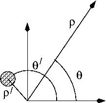
For clarity, we illustrate the expansion for a single line charge, then generalize to an arbitrary distribution of line charges. Through this article, the primed coordinates such as ( ρ ′ , θ ′ ) refer to the position of the line charge(s), whereas the unprimed coordinates such as ( ρ , θ ) refer to the point at which the potential is being observed. We use cylindrical coordinates throughout, e.g., an arbitrary vector r has coordinates ( ρ , θ , z ) where ρ is the radius from the z axis, θ is the azimuthal angle and z is the normal Cartesian coordinate. By assumption, the line charges are infinitely long and aligned with the z axis.
The electric potential of a line charge λ located at ( ρ ′ , θ ′ ) is given by
Φ ( ρ , θ ) = − λ 2 π ϵ ln R = − λ 4 π ϵ ln | ρ 2 + ( ρ ′ ) 2 − 2 ρ ρ ′ cos ( θ − θ ′ ) | where R is the shortest distance between the line charge and the observation point.
By symmetry, the electric potential of an infinite linecharge has no z -dependence. The line charge λ is the charge per unit length in the z -direction, and has units of (charge/length). If the radius ρ of the observation point is greater than the radius ρ ′ of the line charge, we may factor out ρ 2
Φ ( ρ , θ ) = − λ 4 π ϵ { 2 ln ρ + ln ( 1 − ρ ′ ρ e i ( θ − θ ′ ) ) ( 1 − ρ ′ ρ e − i ( θ − θ ′ ) ) } and expand the logarithms in powers of ( ρ ′ / ρ ) < 1
Φ ( ρ , θ ) = − λ 2 π ϵ { ln ρ − ∑ k = 1 ∞ ( 1 k ) ( ρ ′ ρ ) k [ cos k θ cos k θ ′ + sin k θ sin k θ ′ ] } which may be written as
Φ ( ρ , θ ) = − Q 2 π ϵ ln ρ + ( 1 2 π ϵ ) ∑ k = 1 ∞ C k cos k θ + S k sin k θ ρ k where the multipole moments are defined as
Q = λ ,
C k = λ k ( ρ ′ ) k cos k θ ′ ,
and
S k = λ k ( ρ ′ ) k sin k θ ′ .
Conversely, if the radius ρ of the observation point is less than the radius ρ ′ of the line charge, we may factor out ( ρ ′ ) 2 and expand the logarithms in powers of ( ρ / ρ ′ ) < 1
Φ ( ρ , θ ) = − λ 2 π ϵ { ln ρ ′ − ∑ k = 1 ∞ ( 1 k ) ( ρ ρ ′ ) k [ cos k θ cos k θ ′ + sin k θ sin k θ ′ ] } which may be written as
Φ ( ρ , θ ) = − Q 2 π ϵ ln ρ ′ + ( 1 2 π ϵ ) ∑ k = 1 ∞ ρ k [ I k cos k θ + J k sin k θ ] where the interior multipole moments are defined as
Q = λ ,
I k = λ k cos k θ ′ ( ρ ′ ) k ,
and
J k = λ k sin k θ ′ ( ρ ′ ) k .
The generalization to an arbitrary distribution of line charges λ ( ρ ′ , θ ′ ) is straightforward. The functional form is the same
Φ ( r ) = − Q 2 π ϵ ln ρ + ( 1 2 π ϵ ) ∑ k = 1 ∞ C k cos k θ + S k sin k θ ρ k and the moments can be written
Q = ∫ d θ ′ ∫ ρ ′ d ρ ′ λ ( ρ ′ , θ ′ ) C k = ( 1 k ) ∫ d θ ′ ∫ d ρ ′ ( ρ ′ ) k + 1 λ ( ρ ′ , θ ′ ) cos k θ ′ S k = ( 1 k ) ∫ d θ ′ ∫ d ρ ′ ( ρ ′ ) k + 1 λ ( ρ ′ , θ ′ ) sin k θ ′ Note that the λ ( ρ ′ , θ ′ ) represents the line charge per unit area in the ( ρ − θ ) plane.
Similarly, the interior cylindrical multipole expansion has the functional form
Φ ( ρ , θ ) = − Q 2 π ϵ ln ρ ′ + ( 1 2 π ϵ ) ∑ k = 1 ∞ ρ k [ I k cos k θ + J k sin k θ ] where the moments are defined
Q = ∫ d θ ′ ∫ ρ ′ d ρ ′ λ ( ρ ′ , θ ′ ) I k = ( 1 k ) ∫ d θ ′ ∫ d ρ ′ [ cos k θ ′ ( ρ ′ ) k − 1 ] λ ( ρ ′ , θ ′ ) J k = ( 1 k ) ∫ d θ ′ ∫ d ρ ′ [ sin k θ ′ ( ρ ′ ) k − 1 ] λ ( ρ ′ , θ ′ ) A simple formula for the interaction energy of cylindrical multipoles (charge density 1) with a second charge density can be derived. Let f ( r ′ ) be the second charge density, and define λ ( ρ , θ ) as its integral over z
λ ( ρ , θ ) = ∫ d z f ( ρ , θ , z ) The electrostatic energy is given by the integral of the charge multiplied by the potential due to the cylindrical multipoles
U = ∫ d θ ∫ ρ d ρ λ ( ρ , θ ) Φ ( ρ , θ ) If the cylindrical multipoles are exterior, this equation becomes
U = − Q 1 2 π ϵ ∫ ρ d ρ λ ( ρ , θ ) ln ρ + ( 1 2 π ϵ ) ∑ k = 1 ∞ C 1 k ∫ d θ ∫ d ρ [ cos k θ ρ k − 1 ] λ ( ρ , θ ) + ( 1 2 π ϵ ) ∑ k = 1 ∞ S 1 k ∫ d θ ∫ d ρ [ sin k θ ρ k − 1 ] λ ( ρ , θ ) where Q 1 , C 1 k and S 1 k are the cylindrical multipole moments of charge distribution 1. This energy formula can be reduced to a remarkably simple form
U = − Q 1 2 π ϵ ∫ ρ d ρ λ ( ρ , θ ) ln ρ + ( 1 2 π ϵ ) ∑ k = 1 ∞ k ( C 1 k I 2 k + S 1 k J 2 k ) where I 2 k and J 2 k are the interior cylindrical multipoles of the second charge density.
The analogous formula holds if charge density 1 is composed of interior cylindrical multipoles
U = − Q 1 ln ρ ′ 2 π ϵ ∫ ρ d ρ λ ( ρ , θ ) + ( 1 2 π ϵ ) ∑ k = 1 ∞ k ( C 2 k I 1 k + S 2 k J 1 k ) where I 1 k and J 1 k are the interior cylindrical multipole moments of charge distribution 1, and C 2 k and S 2 k are the exterior cylindrical multipoles of the second charge density.
As an example, these formulae could be used to determine the interaction energy of a small protein in the electrostatic field of a double-stranded DNA molecule; the latter is relatively straight and bears a constant linear charge density due to the phosphate groups of its backbone.