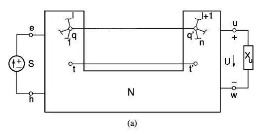
Let e, h, u, w, q=q', and t=t' be six arbitrary nodes of the network N and
S
be an independent voltage or current source connected between e and h, while
U
is the output quantity, either a voltage or current, relative to the branch with immittance
X
u
, connected between u and w. Let us now cut the qq' connection and insert a three-terminal circuit ("TTC") between the two nodes q and q' and the node t=t' , as in figure b (
W
r
and
W
p
are homogeneous quantities, voltages or currents, relative to the ports qt and q'q't' of the TTC).
In order for the two networks N and N' to be equivalent for any
S
, the two constraints
W
r
=
W
p
and
W
r
¯
=
W
p
¯
, where the overline indicates the dual quantity, are to be satisfied.
The above mentioned three-terminal circuit can be implemented, for example, connecting an ideal independent voltage or current source
W
p
between q' and t' , and an immittance
X
p
between q and t.
With reference to the network N', the following network functions can be defined:
A
≡
U
W
p
|
S
=
0
;
β
≡
W
r
U
|
S
=
0
;
X
i
≡
W
p
W
p
¯
|
S
=
0
γ
≡
U
S
|
W
p
=
0
;
α
≡
W
r
S
|
W
p
=
0
;
ρ
≡
W
p
¯
S
|
W
p
=
0
from which, exploiting the Superposition theorem, we obtain:
W
r
=
α
S
+
β
A
W
p
W
p
¯
=
ρ
S
+
W
p
X
i
.
Therefore the first constraint for the equivalence of the networks is satisfied if
W
p
=
α
1
−
β
A
S
.
Furthermore,
W
r
¯
=
W
r
X
p
W
p
¯
=
(
1
X
i
+
ρ
α
(
1
−
β
A
)
)
W
r
therefore the second constraint for the equivalence of the networks holds if
1
X
p
=
1
X
i
+
ρ
α
(
1
−
β
A
)
If we consider the expressions for the network functions
γ
and
A
, the first constraint for the equivalence of the networks, and we also consider that, as a result of the superposition principle,
U
=
γ
S
+
A
W
p
, the transfer function
A
f
≡
U
S
is given by
A
f
=
α
A
1
−
β
A
+
γ
.
For the particular case of a feedback amplifier, the network functions
α
,
γ
and
ρ
take into account the nonidealities of such amplifier. In particular:
α
takes into account the nonideality of the comparison network at the input
γ
takes into account the non unidirectionality of the feedback chain
ρ
takes into account the non unidirectionality of the amplification chain.
If the amplifier can be considered ideal, i.e. if
α
=
1
,
ρ
=
0
and
γ
=
0
, the transfer function reduces to the known expression deriving from classical feedback theory:
A
f
=
A
1
−
β
A
.
Evaluation of the impedance and of the admittance between two nodes
The evaluation of the impedance (or of the admittance) between two nodes is made somewhat simpler by the cut-insertion theorem.
Let us insert a generic source
S
between the nodes j=e=q and k=h between which we want to evaluate the impedance
Z
. By performing a cut as shown in the figure, we notice that the immittance
X
p
is in series with
S
and the current through it is thus the same as that provided by
S
. If we choose an input voltage source
V
s
=
S
and, as a consequence, a current
I
s
=
S
¯
, and an impedance
Z
p
=
X
p
, we can write the following relationships:
Z
=
V
s
I
s
=
V
s
I
r
=
Z
p
V
s
V
r
=
Z
p
V
s
V
p
=
Z
p
1
−
β
A
α
.
Considering that
α
=
V
r
V
s
|
V
p
=
0
=
Z
p
Z
p
+
Z
b
, where
Z
b
is the impedance seen between the nodes k=h and t if remove
Z
p
and short-circuit the voltage sources, we obtain the impedance
Z
between the nodes j and k in the form:
Z
=
(
Z
p
+
Z
b
)
(
1
−
β
A
)
We proceed in a way analogous to the impedance case, but this time the cut will be as shown in the figure to the right, noticing that
S
is now in parallel to
X
p
. If we consider an input current source
I
s
=
S
(as a result we have a voltage
V
s
=
S
¯
) and an admittance
Y
p
=
X
p
, the admittance
Y
between the nodes j and k can be computed as follows:
Y
=
I
s
V
s
=
I
s
V
r
=
Y
p
I
s
I
r
=
Y
p
I
s
I
p
=
Y
p
1
−
β
A
α
.
Considering that
α
=
I
r
I
s
|
I
p
=
0
=
Y
p
Y
p
+
Y
b
, where
Y
b
is the admittance seen between the nodes k=h and t if we remove
Y
p
and open the current sources, we obtain the admittance
Y
in the form:
Y
=
(
Y
p
+
Y
b
)
(
1
−
β
A
)
The implementation of the TTC with an independent source
W
p
and an immittance
X
p
is useful and intuitive for the calculation of the impedance between two nodes, but involves, as in the case of the other network functions, the difficulty of the calculation of
X
p
from the equivalence equation. Such difficulty can be avoided using a dependent source
W
p
¯
in place of
X
p
and using the Blackman formula for the evaluation of
X
. Such an implementation of the TTC allows finding a feedback topology even in a network consisting of a voltage source and two impedances in series.