Cramer's rule

General case

Consider a system of n linear equations for n unknowns, represented in matrix multiplication form as follows:

A x = b

where the n × n matrix A has a nonzero determinant, and the vector x = ( x 1 , … , x n ) T is the column vector of the variables. Then the theorem states that in this case the system has a unique solution, whose individual values for the unknowns are given by:

x i = det ( A i ) det ( A ) i = 1 , … , n

where A i is the matrix formed by replacing the i-th column of A by the column vector b.

A more general version of Cramer's rule considers the matrix equation

A X = B

where the n × n matrix A has a nonzero determinant, and X, B are n × m matrices. Given sequences 1 ≤ i 1 < i 2 < … < i k ≤ n and 1 ≤ j 1 < j 2 < … < j k ≤ m , let X I , J be the k × k submatrix of X with rows in I := ( i 1 , … , i k ) and columns in J := ( j 1 , … , j k ) . Let A B ( I , J ) be the n × n matrix formed by replacing the i s column of A by the j s column of B, for all s = 1 , … , k . Then

det X I , J = det ( A B ( I , J ) ) det ( A ) .

In the case k = 1 , this reduces to the normal Cramer's rule.

The rule holds for systems of equations with coefficients and unknowns in any field, not just in the real numbers. It has recently been shown that Cramer's rule can be implemented in O(n³) time, which is comparable to more common methods of solving systems of linear equations, such as Gaussian elimination (consistently requiring 2.5 times as many arithmetic operations for all matrix sizes, while exhibiting comparable numeric stability in most cases).

Proof

The proof for Cramer's rule uses just two properties of determinants: linearity with respect to any given column (taking for that column a linear combination of column vectors produces as determinant the corresponding linear combination of their determinants), and the fact that the determinant is zero whenever two columns are equal (which is implied by the basic property that the sign of the determinant flips if you switch two columns).

Fix the index j of a column. Linearity means that if we consider only column j as variable (fixing the others arbitrarily), the resulting function Rⁿ → R (assuming matrix entries are in R) can be given by a matrix, with one row and n columns, that acts on column j. In fact this is precisely what Laplace expansion does, writing det(A) = C₁a_1,j + ... + C_na_n,j for certain coefficients C₁, ..., C_n that depend on the columns of A other than column j (the precise expression for these cofactors is not important here). The value det(A) is then the result of applying the one-line matrix L_(j) = (C₁ C₂ ... C_n) to column j of A. If L_(j) is applied to any other column k of A, then the result is the determinant of the matrix obtained from A by replacing column j by a copy of column k, so the resulting determinant is 0 (the case of two equal columns).

Now consider a system of n linear equations in n unknowns x 1 , … , x n , whose coefficient matrix is A, with det(A) assumed to be nonzero:

a 11 x 1 + a 12 x 2 + ⋯ + a 1 n x n = b 1 a 21 x 1 + a 22 x 2 + ⋯ + a 2 n x n = b 2 ⋮ ⋮ ⋮ a n 1 x 1 + a n 2 x 2 + ⋯ + a n n x n = b n .

If one combines these equations by taking C₁ times the first equation, plus C₂ times the second, and so forth until C_n times the last, then the coefficient of x_j will become C₁a_{1, j} + ... + C_na_n,j = det(A), while the coefficients of all other unknowns become 0; the left hand side becomes simply det(A)x_j. The right hand side is C₁b₁ + ... + C_nb_n, which is L_(j) applied to the column vector b of the right hand sides b_i. In fact what has been done here is multiply the matrix equation Ax = b on the left by L_(j). Dividing by the nonzero number det(A) one finds the following equation, necessary to satisfy the system:

x j = L ( j ) ⋅ b det ( A ) .

But by construction the numerator is the determinant of the matrix obtained from A by replacing column j by b, so we get the expression of Cramer's rule as a necessary condition for a solution. The same procedure can be repeated for other values of j to find values for the other unknowns.

The only point that remains to prove is that these values for the unknowns, the only possible ones, do indeed together form a solution. But if the matrix A is invertible with inverse A⁻¹, then x = A⁻¹b will be a solution, thus showing its existence. To see that A is invertible when det(A) is nonzero, consider the n × n matrix M obtained by stacking the one-line matrices L_(j) on top of each other for j = 1, ..., n (this gives the adjugate matrix for A). It was shown that L_(j)A = (0 ... 0 det(A) 0 ... 0) where det(A) appears at the position j; from this it follows that MA = det(A)I_n. Therefore,

1 det ( A ) M = A − 1 ,

completing the proof.

For other proofs, see below.

Finding inverse matrix

Let A be an n × n matrix. Then

A adj ⁡ A = ( adj ⁡ A ) A = det ⁡ ( A ) I

where adj(A) denotes the adjugate matrix of A, det(A) is the determinant, and I is the identity matrix. If det(A) is invertible in R, then the inverse matrix of A is

A − 1 = 1 det ⁡ ( A ) adj ⁡ ( A ) .

If R is a field (such as the field of real numbers), then this gives a formula for the inverse of A, provided det(A) ≠ 0. In fact, this formula will work whenever R is a commutative ring, provided that det(A) is a unit. If det(A) is not a unit, then A is not invertible.

Explicit formulas for small systems

Consider the linear system

{ a 1 x + b 1 y = c 1 a 2 x + b 2 y = c 2

which in matrix format is

[ a 1 b 1 a 2 b 2 ] [ x y ] = [ c 1 c 2 ] .

Assume a₁b₂ − b₁a₂ nonzero. Then, with help of determinants x and y can be found with Cramer's rule as

x = | c 1 b 1 c 2 b 2 | | a 1 b 1 a 2 b 2 | = c 1 b 2 − b 1 c 2 a 1 b 2 − b 1 a 2 , y = | a 1 c 1 a 2 c 2 | | a 1 b 1 a 2 b 2 | = a 1 c 2 − c 1 a 2 a 1 b 2 − b 1 a 2 .

The rules for 3 × 3 matrices are similar. Given

{ a 1 x + b 1 y + c 1 z = d 1 a 2 x + b 2 y + c 2 z = d 2 a 3 x + b 3 y + c 3 z = d 3

which in matrix format is

[ a 1 b 1 c 1 a 2 b 2 c 2 a 3 b 3 c 3 ] [ x y z ] = [ d 1 d 2 d 3 ] .

Then the values of x, y and z can be found as follows:

x = | d 1 b 1 c 1 d 2 b 2 c 2 d 3 b 3 c 3 | | a 1 b 1 c 1 a 2 b 2 c 2 a 3 b 3 c 3 | , y = | a 1 d 1 c 1 a 2 d 2 c 2 a 3 d 3 c 3 | | a 1 b 1 c 1 a 2 b 2 c 2 a 3 b 3 c 3 | ,  and  z = | a 1 b 1 d 1 a 2 b 2 d 2 a 3 b 3 d 3 | | a 1 b 1 c 1 a 2 b 2 c 2 a 3 b 3 c 3 | .

Ricci calculus

Cramer's rule is used in the Ricci calculus in various calculations involving the Christoffel symbols of the first and second kind.

In particular, Cramer's rule can be used to prove that the divergence operator on a Riemannian manifold is invariant with respect to change of coordinates. We give a direct proof, suppressing the role of the Christoffel symbols. Let ( M , g ) be a Riemannian manifold equipped with local coordinates ( x 1 , x 2 , … , x n ) . Let A = A i ∂ ∂ x i be a vector field. We use the summation convention throughout.

Theorem. The divergence of A , div ⁡ A = 1 det g ∂ ∂ x i ( A i det g ) , is invariant under change of coordinates.

Computing derivatives implicitly

Consider the two equations F ( x , y , u , v ) = 0 and G ( x , y , u , v ) = 0 . When u and v are independent variables, we can define x = X ( u , v ) and y = Y ( u , v ) .

Finding an equation for ∂ x ∂ u is a trivial application of Cramer's rule.

Integer programming

Cramer's rule can be used to prove that an integer programming problem whose constraint matrix is totally unimodular and whose right-hand side is integer, has integer basic solutions. This makes the integer program substantially easier to solve.

Ordinary differential equations

Cramer's rule is used to derive the general solution to an inhomogeneous linear differential equation by the method of variation of parameters.

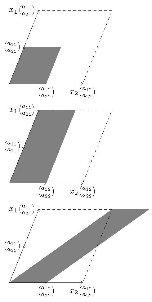
Geometric interpretation

Cramer's rule has a geometric interpretation that can be considered also a proof or simply giving insight about its geometric nature. These geometric arguments work in general and not only in the case of two equations with two unknowns presented here.

Given the system of equations

a 11 x 1 + a 12 x 2 = b 1 a 21 x 1 + a 22 x 2 = b 2

it can be considered as an equation between vectors

x 1 ( a 11 a 21 ) + x 2 ( a 12 a 22 ) = ( b 1 b 2 ) .

The area of the parallelogram determined by ( a 11 a 21 ) and ( a 12 a 22 ) is given by the determinant of the system of equations:

| a 11 a 12 a 21 a 22 | .

In general, when there are more variables and equations, the determinant of n vectors of length n will give the volume of the parallelepiped determined by those vectors in the n-th dimensional Euclidean space.

Therefore, the area of the parallelogram determined by x 1 ( a 11 a 21 ) and ( a 12 a 22 ) has to be x 1 times the area of the first one since one of the sides has been multiplied by this factor. Now, this last parallelogram, by Cavalieri's principle, has the same area as the parallelogram determined by ( b 1 b 2 ) = x 1 ( a 11 a 21 ) + x 2 ( a 12 a 22 ) and ( a 12 a 22 ) .

Equating the areas of this last and the second parallelogram gives the equation

| b 1 a 12 b 2 a 22 | = | a 11 x 1 a 12 a 21 x 1 a 22 | = x 1 | a 11 a 12 a 21 a 22 |

from which Cramer's rule follows.

A short proof

A short proof of Cramer's rule can be given by noticing that x 1 is the determinant of the matrix

X 1 = [ x 1 0 0 … 0 x 2 1 0 … 0 x 3 0 1 … 0 ⋮ ⋮ ⋮ ⋱ ⋮ x n 0 0 … 1 ]

On the other hand, assuming that our original matrix A is invertible, this matrix X 1 has columns A − 1 b , A − 1 v 2 , … , A − 1 v n , where v k is the k-th column of the matrix A. Recall that the matrix A 1 has columns b , v 2 , … , v n . Hence we have

x 1 = det ( X 1 ) = det ( A − 1 ) det ( A 1 ) = det ( A 1 ) det ( A ) .

The proof for other x j is similar.

Proof using Clifford algebra

Consider the system of three scalar equations in three unknown scalars x 1 , x 2 , x 3

a 11 x 1 + a 12 x 2 + a 13 x 3 = c 1 a 21 x 1 + a 22 x 2 + a 23 x 3 = c 2 a 31 x 1 + a 32 x 2 + a 33 x 3 = c 3

and assign an orthonormal vector basis e 1 , e 2 , e 3 for G 3 as

a 11 e 1 x 1 + a 12 e 1 x 2 + a 13 e 1 x 3 = c 1 e 1 a 21 e 2 x 1 + a 22 e 2 x 2 + a 23 e 2 x 3 = c 2 e 2 a 31 e 3 x 1 + a 32 e 3 x 2 + a 33 e 3 x 3 = c 3 e 3

Let the vectors

a 1 = a 11 e 1 + a 21 e 2 + a 31 e 3 a 2 = a 12 e 1 + a 22 e 2 + a 32 e 3 a 3 = a 13 e 1 + a 23 e 2 + a 33 e 3

Adding the system of equations, it is seen that

c = c 1 e 1 + c 2 e 2 + c 3 e 3 = x 1 a 1 + x 2 a 2 + x 3 a 3

Using the exterior product, each unknown scalar x k can be solved as

c ∧ a 2 ∧ a 3 = x 1 a 1 ∧ a 2 ∧ a 3 c ∧ a 1 ∧ a 3 = x 2 a 2 ∧ a 1 ∧ a 3 c ∧ a 1 ∧ a 2 = x 3 a 3 ∧ a 1 ∧ a 2 x 1 = c ∧ a 2 ∧ a 3 a 1 ∧ a 2 ∧ a 3 x 2 = c ∧ a 1 ∧ a 3 a 2 ∧ a 1 ∧ a 3 = a 1 ∧ c ∧ a 3 a 1 ∧ a 2 ∧ a 3 x 3 = c ∧ a 1 ∧ a 2 a 3 ∧ a 1 ∧ a 2 = a 1 ∧ a 2 ∧ c a 1 ∧ a 2 ∧ a 3

For n equations in n unknowns, the solution for the k-th unknown x k generalizes to

x k = a 1 ∧ ⋯ ∧ ( c ) k ∧ ⋯ ∧ a n a 1 ∧ ⋯ ∧ a k ∧ ⋯ ∧ a n = ( a 1 ∧ ⋯ ∧ ( c ) k ∧ ⋯ ∧ a n ) ( a 1 ∧ ⋯ ∧ a k ∧ ⋯ ∧ a n ) − 1 = ( a 1 ∧ ⋯ ∧ ( c ) k ∧ ⋯ ∧ a n ) ( a 1 ∧ ⋯ ∧ a k ∧ ⋯ ∧ a n ) ( a 1 ∧ ⋯ ∧ a k ∧ ⋯ ∧ a n ) ( a 1 ∧ ⋯ ∧ a k ∧ ⋯ ∧ a n ) = ( a 1 ∧ ⋯ ∧ ( c ) k ∧ ⋯ ∧ a n ) ⋅ ( a 1 ∧ ⋯ ∧ a k ∧ ⋯ ∧ a n ) ( − 1 ) n ( n − 1 ) 2 ( a n ∧ ⋯ ∧ a k ∧ ⋯ ∧ a 1 ) ⋅ ( a 1 ∧ ⋯ ∧ a k ∧ ⋯ ∧ a n ) = ( a n ∧ ⋯ ∧ ( c ) k ∧ ⋯ ∧ a 1 ) ⋅ ( a 1 ∧ ⋯ ∧ a k ∧ ⋯ ∧ a n ) ( a n ∧ ⋯ ∧ a k ∧ ⋯ ∧ a 1 ) ⋅ ( a 1 ∧ ⋯ ∧ a k ∧ ⋯ ∧ a n )

If a_k are linearly independent, then the x k can be expressed in determinant form identical to Cramer’s Rule as

x k = ( a n ∧ ⋯ ∧ ( c ) k ∧ ⋯ ∧ a 1 ) ⋅ ( a 1 ∧ ⋯ ∧ a k ∧ ⋯ ∧ a n ) ( a n ∧ ⋯ ∧ a k ∧ ⋯ ∧ a 1 ) ⋅ ( a 1 ∧ ⋯ ∧ a k ∧ ⋯ ∧ a n ) = | a 1 ⋅ a 1 ⋯ a 1 ⋅ ( c ) k ⋯ a 1 ⋅ a n ⋮ ⋱ ⋮ ⋱ ⋮ a k ⋅ a 1 ⋯ a k ⋅ ( c ) k ⋯ a k ⋅ a n ⋮ ⋱ ⋮ ⋱ ⋮ a n ⋅ a 1 ⋯ a n ⋅ ( c ) k ⋯ a n ⋅ a n | | a 1 ⋅ a 1 ⋯ a 1 ⋅ a k ⋯ a 1 ⋅ a n ⋮ ⋱ ⋮ ⋱ ⋮ a k ⋅ a 1 ⋯ a k ⋅ a k ⋯ a k ⋅ a n ⋮ ⋱ ⋮ ⋱ ⋮ a n ⋅ a 1 ⋯ a n ⋅ a k ⋯ a n ⋅ a n | − 1 = | a 1 ⋮ a k ⋮ a n | | a 1 ⋯ ( c ) k ⋯ a n | | a 1 ⋮ a k ⋮ a n | − 1 | a 1 ⋯ a k ⋯ a n | − 1 = | a 1 ⋯ ( c ) k ⋯ a n | | a 1 ⋯ a k ⋯ a n | − 1 = | a 11 … c 1 ⋯ a 1 n ⋮ ⋱ ⋮ ⋱ ⋮ a k 1 ⋯ c k ⋯ a k n ⋮ ⋱ ⋮ ⋱ ⋮ a n 1 ⋯ c n ⋯ a n n | | a 11 … a 1 k ⋯ a 1 n ⋮ | − 1

where (c)_k denotes the substitution of vector a_k with vector c in the k-th numerator position.

Incompatible and indeterminate cases

A system of equations is said to be incompatible or inconsistent when there are no solutions and it is called indeterminate when there is more than one solution. For linear equations, an indeterminate system will have infinitely many solutions (if it is over an infinite field), since the solutions can be expressed in terms of one or more parameters that can take arbitrary values.

Cramer's rule applies to the case where the coefficient determinant is nonzero. In the 2×2 case, if the coefficient determinant is zero, then the system is incompatible if the numerator determinants are nonzero, or indeterminate if the numerator determinants are zero.

For 3×3 or higher systems, the only thing one can say when the coefficient determinant equals zero is that if any of the numerator determinants are nonzero, then the system must be incompatible. However, having all determinants zero does not imply that the system is indeterminate. A simple example where all determinants vanish (equal zero) but the system is still incompatible is the 3×3 system x+y+z=1, x+y+z=2, x+y+z=3.