Covariance mapping

Simple covariance mapping

Covariance mapping can be applied to any repetitive, fluctuating signal to reveal information hidden in the fluctuations. This technique was first used to analyse mass spectra of molecules ionised and fragmented by intense laser pulses.

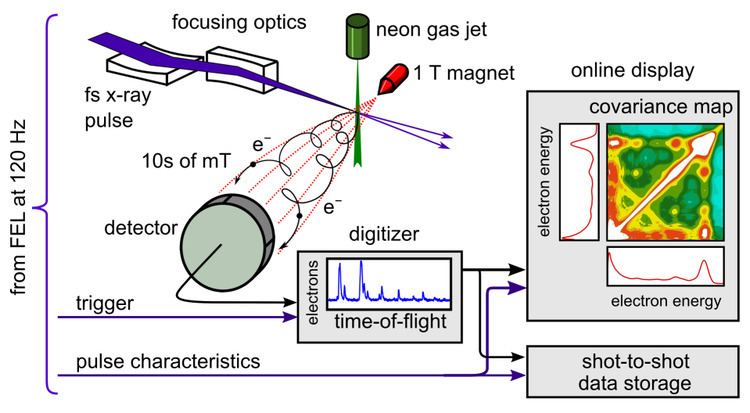
Covariance mapping is particularly well suited to free-electron laser (FEL) research, where the x-ray intensity is so high that the large number of photoelectron and photoions produced at each pulse overwhelms simpler coincidence techniques. Figure 1 shows a typical experiment. X-ray pulses are focused on neon atoms and ionise them. The kinetic energy spectra of the photoelectrons ejected from neon are recorded at each laser shot using a suitable spectrometer (here a time-of-flight spectrometer). The single-shot spectra are sent to a computer, which calculates and displays the covariance map.

The need for correlations

Even in a relatively simple system, such as the neon atom, intense x-rays induce a plethora of ionisation processes (see Fig. 2). As the kinetic energies of the electrons ejected in different processes largely overlap, it is impossible to identify these processes using simple photoelectron spectrometry. To do so, one needs to correlate the kinetic energies of the electrons ejected in a given process. Covariance mapping is a method of revealing such correlations.

The principle

Consider a random function X n ( E ) , where index n labels a particular instance of the function and E is the independent variable. In the context of the FEL experiment, X n ( E ) is a digitized electron energy spectrum produced by laser shot n . As the electron energy E takes a range of discrete values E i in places where the spectrum is sampled, the spectra can be regarded as row vectors of experimental data:

The simplest way to analyse the data is to average the spectra over N laser shots:

Such spectra show kinetic energies of individual electrons but the correlations between the electrons are lost in the process of averaging. To reveal the correlations we need to calculate the covariance map:

where vector Y is the transpose of vector X and the angular brackets denote averaging over many laser shots as before. Note that the ordering of the vectors (a column followed by a row) ensures that their multiplication gives a matrix. It is convenient to display the matrix as a false-colour map.

How to read the map

The covariance map obtained in the FEL experiment is shown in Fig. 3. Along the x and y axes the averaged spectra ⟨ X ⟩ and ⟨ Y ⟩ are shown. These spectra are resolved on the map into pairwise correlations between energies of electrons coming from the same process. For example, if the process is the first process depicted in Fig. 2 (PP), then two low-energy electrons are ejected from the Ne core giving a positive island in the bottom-left corner of the map (one of the white ones). The island is positive because if one of the electrons is detected, there is higher than average probability of detecting also the other electron and the covariance of the signals at the two energies takes a positive value.

The volumes of the islands are directly proportional to the relative probabilities of the ionisation processes. This useful quality of the map follows from a property of the Poisson distribution, which governs the number of neon atoms in the focal volume and the number of electrons produced at a particular energy, X n ( E i ) . The property employed here is that the variance of a Poisson distribution is equal to its mean and this property is also inherited by covariance. Therefore the covariance plotted on the map is proportional to the number of neon atoms that produce pairs of electrons of particular energies. This makes covariance much more suitable for particle counting experiments than other bivariate estimators, such as Pearson's correlation coefficient.

On the diagonal of the map there is an autocorrelation line. It is present there because the same spectra are used for the x and y axes. Thus, if an electron pulse is present at a particular energy on one axis, it is also present on the other axis giving the variance signal along the E x = E y line, which is usually stronger than the neighbouring covariance islands. The mirror symmetry of the map with respect to this line has the same origin. The autocorrelation line and the mirror symmetry are not present if two different detectors are used for the x and y signals, for example where one detector is used to detect ions and another to detect electrons.

Much more information is present on the map than on the averaged, 1D spectrum. The single, often broad and indistinct peaks on the 1D spectrum are resolved into several islands on the map. Fig. 4 shows magnified core-core and core-valence regions with several ionisation sequences identified unambiguously. In the D_KV process the two electrons ejected share arbitrarily the energy available from a single proton producing a conspicuous line E_x + E_y = const in the left panel of Fig. 4. Impurities, such as water vapour or nitrogen, give islands usually away from the islands of the species studied (see Fig. 3b,e,f).

Partial covariance mapping

Covariance maps expose all kinds of correlations, including indirect ones that are induced by a fluctuating common parameter. Such common-mode correlations are often uninteresting and they obscure the interesting ones. For example, in the laser experiments the pulse intensity may fluctuate from shot to shot. These fluctuations correlate every electron with every other electron, simply because a more intense pulse produces more electrons of every energy.

Removal of uninteresting correlations

The influence of such uninteresting correlations can be removed using partial covariance mapping. This method exposes only a part of the correlations, the part that is independent of the fluctuating parameter I , which has to be measured at every laser shot. The formula for partial covariance is

where cov ⁡ ( I , I ) is the variance of the fluctuating parameter.

Stages of partial covariance mapping

It is instructive to see how this formula works on an example of another experiment performed at the FLASH FEL in Hamburg. (In fact this method was also used to analyse the LCLS experiment described above, but to keep the Wikipedia description simple the partial covariance was not mentioned.) The FLASH experimental setup was very similar to the LCLS setup shown in Fig. 1, except molecular nitrogen was studied and its ions rather than electrons were detected. Fig. 5a shows the correlated product ⟨ Y X ⟩ and Fig. 5b shows the uncorrelated product ⟨ Y ⟩ ⟨ X ⟩ . Their difference gives the simple covariance map (c). The momentum correlation lines start to be visible (note a change in the colour scale) but the map is overwhelmed by correlations induced by FEL intensity fluctuations. These correlations are calculated in panel (d) and the correction is subtracted from map (c) giving map (e). The momentum correlation lines are now clearly visible but some residual common-mode background is still present, which is likely to be induced by other fluctuating parameters, such as the sample density or the FEL pulse duration. As these parameters were not monitored, simply an excess of the correction (d) was subtracted from map (e) giving map (f). This crude, ad hoc method significantly suppresses the residual common-mode background in the region of interest but the overcorrection introduces negative regions (magenta) at long time of flights. The detailed algorithm of partial covariance mapping is given in the Supplemental Material of the LCLS paper.

Other reading