Correlation and dependence

Pearson's product-moment coefficient

The most familiar measure of dependence between two quantities is the Pearson product-moment correlation coefficient, or "Pearson's correlation coefficient", commonly called simply "the correlation coefficient". It is obtained by dividing the covariance of the two variables by the product of their standard deviations. Karl Pearson developed the coefficient from a similar but slightly different idea by Francis Galton.

The population correlation coefficient ρ_X,Y between two random variables X and Y with expected values μ_X and μ_Y and standard deviations σ_X and σ_Y is defined as:

where E is the expected value operator, cov means covariance, and corr is a widely used alternative notation for the correlation coefficient.

The Pearson correlation is defined only if both of the standard deviations are finite and nonzero. It is a corollary of the Cauchy–Schwarz inequality that the correlation cannot exceed 1 in absolute value. The correlation coefficient is symmetric: corr(X,Y) = corr(Y,X).

The Pearson correlation is +1 in the case of a perfect direct (increasing) linear relationship (correlation), −1 in the case of a perfect decreasing (inverse) linear relationship (anticorrelation), and some value in the open interval (−1, 1) in all other cases, indicating the degree of linear dependence between the variables. As it approaches zero there is less of a relationship (closer to uncorrelated). The closer the coefficient is to either −1 or 1, the stronger the correlation between the variables.

If the variables are independent, Pearson's correlation coefficient is 0, but the converse is not true because the correlation coefficient detects only linear dependencies between two variables. For example, suppose the random variable X is symmetrically distributed about zero, and Y = X². Then Y is completely determined by X, so that X and Y are perfectly dependent, but their correlation is zero; they are uncorrelated. However, in the special case when X and Y are jointly normal, uncorrelatedness is equivalent to independence.

If we have a series of n measurements of X and Y written as x_i and y_i for i = 1, 2, ..., n, then the sample correlation coefficient can be used to estimate the population Pearson correlation r between X and Y. The sample correlation coefficient is written:

where x and y are the sample means of X and Y, and s_x and s_y are the sample standard deviations of X and Y.

This can also be written as:

If x and y are results of measurements that contain measurement error, the realistic limits on the correlation coefficient are not −1 to +1 but a smaller range.

For the case of a linear model with a single independent variable, the coefficient of determination (R squared) is the square of r, Pearson's product-moment coefficient.

Rank correlation coefficients

Rank correlation coefficients, such as Spearman's rank correlation coefficient and Kendall's rank correlation coefficient (τ) measure the extent to which, as one variable increases, the other variable tends to increase, without requiring that increase to be represented by a linear relationship. If, as the one variable increases, the other decreases, the rank correlation coefficients will be negative. It is common to regard these rank correlation coefficients as alternatives to Pearson's coefficient, used either to reduce the amount of calculation or to make the coefficient less sensitive to non-normality in distributions. However, this view has little mathematical basis, as rank correlation coefficients measure a different type of relationship than the Pearson product-moment correlation coefficient, and are best seen as measures of a different type of association, rather than as alternative measure of the population correlation coefficient.

To illustrate the nature of rank correlation, and its difference from linear correlation, consider the following four pairs of numbers (x, y):

As we go from each pair to the next pair x increases, and so does y. This relationship is perfect, in the sense that an increase in x is always accompanied by an increase in y. This means that we have a perfect rank correlation, and both Spearman's and Kendall's correlation coefficients are 1, whereas in this example Pearson product-moment correlation coefficient is 0.7544, indicating that the points are far from lying on a straight line. In the same way if y always decreases when x increases, the rank correlation coefficients will be −1, while the Pearson product-moment correlation coefficient may or may not be close to −1, depending on how close the points are to a straight line. Although in the extreme cases of perfect rank correlation the two coefficients are both equal (being both +1 or both −1), this is not generally the case, and so values of the two coefficients cannot meaningfully be compared. For example, for the three pairs (1, 1) (2, 3) (3, 2) Spearman's coefficient is 1/2, while Kendall's coefficient is 1/3.

Other measures of dependence among random variables

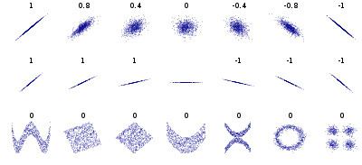
The information given by a correlation coefficient is not enough to define the dependence structure between random variables. The correlation coefficient completely defines the dependence structure only in very particular cases, for example when the distribution is a multivariate normal distribution. (See diagram above.) In the case of elliptical distributions it characterizes the (hyper-)ellipses of equal density, however, it does not completely characterize the dependence structure (for example, a multivariate t-distribution's degrees of freedom determine the level of tail dependence).

Distance correlation was introduced to address the deficiency of Pearson's correlation that it can be zero for dependent random variables; zero distance correlation implies independence.

The Randomized Dependence Coefficient is a computationally efficient, copula-based measure of dependence between multivariate random variables. RDC is invariant with respect to non-linear scalings of random variables, is capable of discovering a wide range of functional association patterns and takes value zero at independence.

The correlation ratio is able to detect almost any functional dependency, and the entropy-based mutual information, total correlation and dual total correlation are capable of detecting even more general dependencies. These are sometimes referred to as multi-moment correlation measures, in comparison to those that consider only second moment (pairwise or quadratic) dependence.

The polychoric correlation is another correlation applied to ordinal data that aims to estimate the correlation between theorised latent variables.

One way to capture a more complete view of dependence structure is to consider a copula between them.

The coefficient of determination generalizes the correlation coefficient for relationships beyond simple linear regression.

Sensitivity to the data distribution

The degree of dependence between variables X and Y does not depend on the scale on which the variables are expressed. That is, if we are analyzing the relationship between X and Y, most correlation measures are unaffected by transforming X to a + bX and Y to c + dY, where a, b, c, and d are constants (b and d being positive). This is true of some correlation statistics as well as their population analogues. Some correlation statistics, such as the rank correlation coefficient, are also invariant to monotone transformations of the marginal distributions of X and/or Y.

Most correlation measures are sensitive to the manner in which X and Y are sampled. Dependencies tend to be stronger if viewed over a wider range of values. Thus, if we consider the correlation coefficient between the heights of fathers and their sons over all adult males, and compare it to the same correlation coefficient calculated when the fathers are selected to be between 165 cm and 170 cm in height, the correlation will be weaker in the latter case. Several techniques have been developed that attempt to correct for range restriction in one or both variables, and are commonly used in meta-analysis; the most common are Thorndike's case II and case III equations.

Various correlation measures in use may be undefined for certain joint distributions of X and Y. For example, the Pearson correlation coefficient is defined in terms of moments, and hence will be undefined if the moments are undefined. Measures of dependence based on quantiles are always defined. Sample-based statistics intended to estimate population measures of dependence may or may not have desirable statistical properties such as being unbiased, or asymptotically consistent, based on the spatial structure of the population from which the data were sampled.

Sensitivity to the data distribution can be used to an advantage. For example, scaled correlation is designed to use the sensitivity to the range in order to pick out correlations between fast components of time series. By reducing the range of values in a controlled manner, the correlations on long time scale are filtered out and only the correlations on short time scales are revealed.

Correlation matrices

The correlation matrix of n random variables X₁, ..., X_n is the n  ×  n matrix whose i,j entry is corr(X_i, X_j). If the measures of correlation used are product-moment coefficients, the correlation matrix is the same as the covariance matrix of the standardized random variables X_i / σ (X_i) for i = 1, ..., n. This applies to both the matrix of population correlations (in which case "σ" is the population standard deviation), and to the matrix of sample correlations (in which case "σ" denotes the sample standard deviation). Consequently, each is necessarily a positive-semidefinite matrix. Moreover, the correlation matrix is strictly positive definite if no variable can have all its values exactly generated as a linear combination of the others.

The correlation matrix is symmetric because the correlation between X_i and X_j is the same as the correlation between X_j and X_i.

A correlation matrix appears, for example, in one formula for the coefficient of multiple determination, a measure of goodness of fit in multiple regression.

Correlation and causality

The conventional dictum that "correlation does not imply causation" means that correlation cannot be used to infer a causal relationship between the variables. This dictum should not be taken to mean that correlations cannot indicate the potential existence of causal relations. However, the causes underlying the correlation, if any, may be indirect and unknown, and high correlations also overlap with identity relations (tautologies), where no causal process exists. Consequently, establishing a correlation between two variables is not a sufficient condition to establish a causal relationship (in either direction).

A correlation between age and height in children is fairly causally transparent, but a correlation between mood and health in people is less so. Does improved mood lead to improved health, or does good health lead to good mood, or both? Or does some other factor underlie both? In other words, a correlation can be taken as evidence for a possible causal relationship, but cannot indicate what the causal relationship, if any, might be.

Correlation and linearity

The Pearson correlation coefficient indicates the strength of a linear relationship between two variables, but its value generally does not completely characterize their relationship. In particular, if the conditional mean of Y given X, denoted E(Y | X), is not linear in X, the correlation coefficient will not fully determine the form of E(Y | X).

The image on the right shows scatter plots of Anscombe's quartet, a set of four different pairs of variables created by Francis Anscombe. The four y variables have the same mean (7.5), variance (4.12), correlation (0.816) and regression line (y = 3 + 0.5x). However, as can be seen on the plots, the distribution of the variables is very different. The first one (top left) seems to be distributed normally, and corresponds to what one would expect when considering two variables correlated and following the assumption of normality. The second one (top right) is not distributed normally; while an obvious relationship between the two variables can be observed, it is not linear. In this case the Pearson correlation coefficient does not indicate that there is an exact functional relationship: only the extent to which that relationship can be approximated by a linear relationship. In the third case (bottom left), the linear relationship is perfect, except for one outlier which exerts enough influence to lower the correlation coefficient from 1 to 0.816. Finally, the fourth example (bottom right) shows another example when one outlier is enough to produce a high correlation coefficient, even though the relationship between the two variables is not linear.

These examples indicate that the correlation coefficient, as a summary statistic, cannot replace visual examination of the data. Note that the examples are sometimes said to demonstrate that the Pearson correlation assumes that the data follow a normal distribution, but this is not correct.

Bivariate normal distribution

If a pair (X, Y) of random variables follows a bivariate normal distribution, the conditional mean E(X|Y) is a linear function of Y, and the conditional mean E(Y|X) is a linear function of X. The correlation coefficient r between X and Y, along with the marginal means and variances of X and Y, determines this linear relationship:

where E ( X ) and E ( Y ) are the expected values of X and Y, respectively, and σ_x and σ_y are the standard deviations of X and Y, respectively.