Copula (probability theory)

Mathematical definition

Consider a random vector ( X 1 , X 2 , … , X d ) . Suppose its marginals are continuous, i.e. the marginal CDFs F i ( x ) = P [ X i ≤ x ] are continuous functions. By applying the probability integral transform to each component, the random vector

has uniformly distributed marginals.

The copula of ( X 1 , X 2 , … , X d ) is defined as the joint cumulative distribution function of ( U 1 , U 2 , … , U d ) :

The copula C contains all information on the dependence structure between the components of ( X 1 , X 2 , … , X d ) whereas the marginal cumulative distribution functions F i contain all information on the marginal distributions.

The importance of the above is that the reverse of these steps can be used to generate pseudo-random samples from general classes of multivariate probability distributions. That is, given a procedure to generate a sample ( U 1 , U 2 , … , U d ) from the copula distribution, the required sample can be constructed as

The inverses F i − 1 are unproblematic as the F i were assumed to be continuous. The above formula for the copula function can be rewritten to correspond to this as:

Definition

In probabilistic terms, C : [ 0 , 1 ] d → [ 0 , 1 ] is a d-dimensional copula if C is a joint cumulative distribution function of a d-dimensional random vector on the unit cube [ 0 , 1 ] d with uniform marginals.

In analytic terms, C : [ 0 , 1 ] d → [ 0 , 1 ] is a d-dimensional copula if

For instance, in the bivariate case, C : [ 0 , 1 ] × [ 0 , 1 ] → [ 0 , 1 ] is a bivariate copula if C ( 0 , u ) = C ( u , 0 ) = 0 , C ( 1 , u ) = C ( u , 1 ) = u and C ( u 2 , v 2 ) − C ( u 2 , v 1 ) − C ( u 1 , v 2 ) + C ( u 1 , v 1 ) ≥ 0 for all 0 ≤ u 1 ≤ u 2 ≤ 1 and 0 ≤ v 1 ≤ v 2 ≤ 1 .

Sklar's theorem

Sklar's theorem, named after Abe Sklar, provides the theoretical foundation for the application of copulas. Sklar's theorem states that every multivariate cumulative distribution function

of a random vector ( X 1 , X 2 , … , X d ) can be expressed in terms of its marginals F i ( x ) = P [ X i ≤ x ] and a copula C . Indeed:

In case that the multivariate distribution has a density h , and this is available, it holds further that

where c is the density of the copula.

The theorem also states that, given H , the copula is unique on Ran ⁡ ( F 1 ) × ⋯ × Ran ⁡ ( F d ) , which is the cartesian product of the ranges of the marginal cdf's. This implies that the copula is unique if the marginals F i are continuous.

The converse is also true: given a copula C : [ 0 , 1 ] d → [ 0 , 1 ] and margins F i ( x ) then C ( F 1 ( x 1 ) , … , F d ( x d ) ) defines a d-dimensional cumulative distribution function.

Fréchet–Hoeffding copula bounds

The Fréchet–Hoeffding Theorem (after Maurice René Fréchet and Wassily Hoeffding ) states that for any Copula C : [ 0 , 1 ] d → [ 0 , 1 ] and any ( u 1 , … , u d ) ∈ [ 0 , 1 ] d the following bounds hold:

The function W is called lower Fréchet–Hoeffding bound and is defined as

The function M is called upper Fréchet–Hoeffding bound and is defined as

The upper bound is sharp: M is always a copula, it corresponds to comonotone random variables.

The lower bound is point-wise sharp, in the sense that for fixed u, there is a copula C ~ such that C ~ ( u ) = W ( u ) . However, W is a copula only in two dimensions, in which case it corresponds to countermonotonic random variables.

In two dimensions, i.e. the bivariate case, the Fréchet–Hoeffding Theorem states

Families of copulas

Several families of copulae have been described.

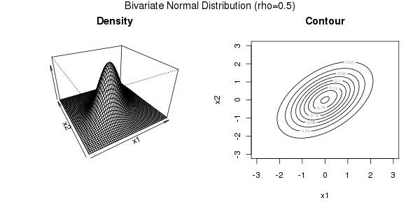
Gaussian copula

The Gaussian copula is a distribution over the unit cube [ 0 , 1 ] d . It is constructed from a multivariate normal distribution over R d by using the probability integral transform.

For a given correlation matrix R ∈ [ − 1 , 1 ] d × d , the Gaussian copula with parameter matrix R can be written as

where Φ − 1 is the inverse cumulative distribution function of a standard normal and Φ R is the joint cumulative distribution function of a multivariate normal distribution with mean vector zero and covariance matrix equal to the correlation matrix R . While there is no simple analytical formula for the copula function, C R Gauss ( u ) , it can be upper or lower bounded, and approximated using numerical integration. The density can be written as

where I is the identity matrix.

Archimedean copulas

Archimedean copulas are an associative class of copulas. Most common Archimedean copulas admit an explicit formula, something not possible for instance for the Gaussian copula. In practice, Archimedean copulas are popular because they allow modeling dependence in arbitrarily high dimensions with only one parameter, governing the strength of dependence.

A copula C is called Archimedean if it admits the representation

where ψ : [ 0 , 1 ] × Θ → [ 0 , ∞ ) is a continuous, strictly decreasing and convex function such that ψ ( 1 ; θ ) = 0 . θ is a parameter within some parameter space Θ . ψ is the so-called generator function and ψ [ − 1 ] is its pseudo-inverse defined by

Moreover, the above formula for C yields a copula for ψ − 1 if and only if ψ − 1 is d-monotone on [ 0 , ∞ ) . That is, if it is d − 2 times differentiable and the derivatives satisfy

for all t ≥ 0 and k = 0 , 1 , … , d − 2 and ( − 1 ) d − 2 ψ − 1 , ( d − 2 ) ( t ; θ ) is nonincreasing and convex.

Most important Archimedean copulas

The following tables highlight the most prominent bivariate Archimedean copulas, with their corresponding generator. Note that not all of them are completely monotone, i.e. d-monotone for all d ∈ N or d-monotone for certain θ ∈ Θ only.

Expectation for copula models and Monte Carlo integration

In statistical applications, many problems can be formulated in the following way. One is interested in the expectation of a response function g : R d → R applied to some random vector ( X 1 , … , X d ) . If we denote the cdf of this random vector with H , the quantity of interest can thus be written as

If H is given by a copula model, i.e.,

this expectation can be rewritten as

In case the copula C is absolutely continuous, i.e. C has a density c, this equation can be written as

and if each marginal distribution has the density f i it holds further that

If copula and margins are known (or if they have been estimated), this expectation can be approximated through the following Monte Carlo algorithm:

1. Draw a sample ( U 1 k , … , U d k ) ∼ C ( k = 1 , … , n ) of size n from the copula C
2. By applying the inverse marginal cdf's, produce a sample of ( X 1 , … , X d ) by setting ( X 1 k , … , X d k ) = ( F 1 − 1 ( U 1 k ) , … , F d − 1 ( U d k ) ) ∼ H ( k = 1 , … , n )
3. Approximate E [ g ( X 1 , … , X d ) ] by its empirical value:

Empirical copulas

When studying multivariate data, one might want to investigate the underlying copula. Suppose we have observations

from a random vector ( X 1 , X 2 , … , X d ) with continuous margins. The corresponding "true" copula observations would be

However, the marginal distribution functions F i are usually not known. Therefore, one can construct pseudo copula observations by using the empirical distribution functions

instead. Then, the pseudo copula observations are defined as

The corresponding empirical copula is then defined as

The components of the pseudo copula samples can also be written as U ~ k i = R k i / n , where R k i is the rank of the observation X k i :

Therefore, the empirical copula can be seen as the empirical distribution of the rank transformed data.

Quantitative finance

In risk/portfolio management, copulas are used to perform stress-tests and robustness checks that are especially important during “downside/crisis/panic regimes” where extreme downside events may occur (e.g., the global financial crisis of 2007–2008).

The formula was also adapted for financial markets and was used to estimate the probability distribution of losses on pools of loans or bonds. The users of the formula have been criticized for creating "evaluation cultures" that continued to use simple copulæ despite the simple versions being acknowledged as inadequate for that purpose. During a downside regime, a large number of investors who have held positions in riskier assets such as equities or real estate may seek refuge in ‘safer’ investments such as cash or bonds. This is also known as a flight-to-quality effect and investors tend to exit their positions in riskier assets in large numbers in a short period of time. As a result, during downside regimes, correlations across equities are greater on the downside as opposed to the upside and this may have disastrous effects on the economy. For example, anecdotally, we often read financial news headlines reporting the loss of hundreds of millions of dollars on the stock exchange in a single day; however, we rarely read reports of positive stock market gains of the same magnitude and in the same short time frame.

Copulas are useful in portfolio/risk management and help us analyse the effects of downside regimes by allowing the modelling of the marginals and dependence structure of a multivariate probability model separately. For example, consider the stock exchange as a market consisting of a large number of traders each operating with his/her own strategies to maximize profits. The individualistic behaviour of each trader can be described by modelling the marginals. However, as all traders operate on the same exchange, each trader's actions have an interaction effect with other traders'. This interaction effect can be described by modelling the dependence structure. Therefore, copulas allow us to analyse the interaction effects which are of particular interest during downside regimes as investors tend to herd their trading behaviour and decisions.

Previously, scalable copula models for large dimensions only allowed the modelling of elliptical dependence structures (i.e., Gaussian and Student-t copulas) that do not allow for correlation asymmetries where correlations differ on the upside or downside regimes. However, the recent development of vine copulas (also known as pair copulas) enables the flexible modelling of the dependence structure for portfolios of large dimensions. The Clayton canonical vine copula allows for the occurrence of extreme downside events and has been successfully applied in portfolio choice and risk management applications. The model is able to reduce the effects of extreme downside correlations and produces improved statistical and economic performance compared to scalable elliptical dependence copulas such as the Gaussian and Student-t copula. Other models developed for risk management applications are panic copulas that are glued with market estimates of the marginal distributions to analyze the effects of panic regimes on the portfolio profit and loss distribution. Panic copulas are created by Monte Carlo simulation, mixed with a re-weighting of the probability of each scenario.

As far as derivatives pricing is concerned, dependence modelling with copula functions is widely used in applications of financial risk assessment and actuarial analysis – for example in the pricing of collateralized debt obligations (CDOs). Some believe the methodology of applying the Gaussian copula to credit derivatives to be one of the reasons behind the global financial crisis of 2008–2009. Despite this perception, there are documented attempts of the financial industry, occurring before the crisis, to address the limitations of the Gaussian copula and of copula functions more generally, specifically the lack of dependence dynamics. The Gaussian copula is lacking as it only allows for an elliptical dependence structure, as dependence is only modeled using the variance-covariance matrix. This methodology is limited such that it does not allow for dependence to evolve as the financial markets exhibit asymmetric dependence, whereby correlations across assets significantly increase during downturns compared to upturns. Therefore, modeling approaches using the Gaussian copula exhibit a poor representation of extreme events. There have been attempts to propose models rectifying some of the copula limitations.

While the application of copulas in credit has gone through popularity as well as misfortune during the global financial crisis of 2008–2009, it is arguably an industry standard model for pricing CDOs. Copulas have also been applied to other asset classes as a flexible tool in analyzing multi-asset derivative products. The first such application outside credit was to use a copula to construct an implied basket volatility surface, taking into account the volatility smile of basket components. Copulas have since gained popularity in pricing and risk management of options on multi-assets in the presence of volatility smile/skew, in equity, foreign exchange and fixed income derivative business. Some typical example applications of copulas are listed below:

Civil engineering

Recently, copula functions have been successfully applied to the database formulation for the reliability analysis of highway bridges, and to various multivariate simulation studies in civil, mechanical and offshore engineering. Researchers are also trying these functions in field of transportation to understand interaction of individual driver behavior components which in totality shapes up the nature of an entire traffic flow.

Reliability engineering

Copulas are being used for reliability analysis of complex systems of machine components with competing failure modes.

Warranty data analysis

Copulas are being used for warranty data analysis in which the tail dependence is analysed

Turbulent combustion

Copulas are used in modelling turbulent partially premixed combustion, which is common in practical combustors.

Medicine

Copula functions have been successfully applied to the analysis of neuronal dependencies and spike counts in neuroscience

Climate and weather research

Copulas have been extensively used in climate- and weather-related research.

Random vector generation

Large synthetic traces of vectors and stationary time series can be generated using empirical copula while preserving the entire dependence structure of small datasets. Such empirical traces are useful in various simulation-based performance studies.