
 | ||
One of the causes of attenuation of radio propagation is the absorption by the atmosphere. There are many well known facts on the phenomenon and qualitative treatments in textbooks. A document published by the International Telecommunication Union (ITU) provides some basis for a quantitative assessment of the attenuation. That document describes a simplified model along with semi-empirical formulas based on data fitting. It also recommended an algorithm to compute the attenuation of radiowave propagation in the atmosphere. NASA also published a study on a related subject. Free software from CNES based on ITU-R recommendations is available for download and is available to the public.
Contents
The model and the ITU recommendation
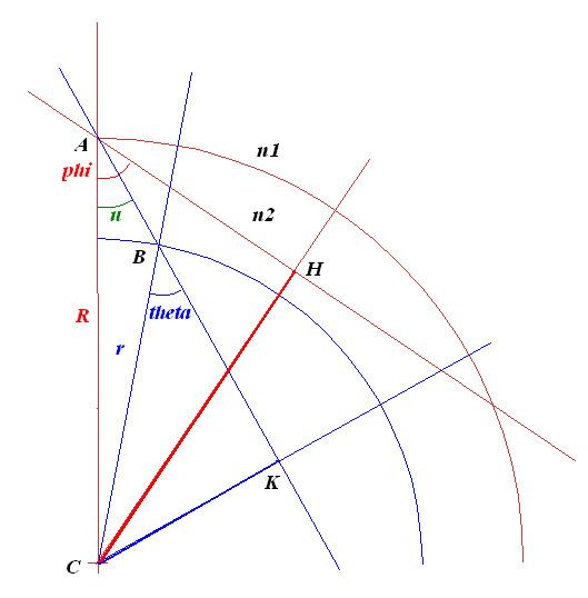
The document ITU-R P.676-8 of the ITU-R section considers the atmosphere as being divided into spherical homogeneous layers; each layer has a constant refraction index. By the use of trigonometry, a couple of formulas and an algorithm were derived.
Through the use of an invariant, the same results can be directly derived:
An incident ray at A under the angle Φ hits the layer B at the angle θ. From basic Euclidean geometry:
By Snell's law:
so that
Notes:
The ITU recommended algorithm consists of launching a ray from a radio source, then at each step, a layer is chosen and a new incidence angle is then computed. The process is iterated until the altitude of the target is reached. At each step, the covered distance dL is multiplied by a specific attenuation coefficient g expressed in dB/km. All the increments g dL are added to provide the total attenuation.
Note that the algorithm does not guaranty that the target is actually reached. For this, a much harder boundary value problem would have to be solved.
The eikonal equation
This equation is discussed in the references. The equation is highly non-linear. Given that a smooth data fitting curve n(altitude) is provided by the ITU for the refraction index n, and that the values of n differs from 1 only by something of the order 10−4, a numerical solution of the eikonal equation can be considered. Usually the equation is presented under the self-adjoint form, a more tractable equation for the ray head position vector r is given in generic parametric form:
Implementations
Three implementations to compute the attenuations exist:
The first two are only of 1st order approximation (see Orders of approximation). For the eikonal equation, many numerical schemes are available. Here only a simple second order scheme was chosen. For most standard configurations of source-target, the three methods differ little from each other. It is only in the case of rays grazing the ground that the differences are meaningful. The following was used for testing:
At the latitude of 10°, when a ray starts at 5 km altitude with an elevation angle of −1° to hit a target at the same longitude but at latitude 8.84° and altitude 30 km. At 22.5 GHz, the results are:
Note that 22.5 GHz is not a practical frequency but it is the most suitable for algorithms comparison. In the table, the first column gives the results in dB, the third gives the distance covered and the last gives the final altitude. Distances are in km. From the altitude 30 km up, the attenuation is negligible. The paths of the three are plotted:
The linear path is the highest on the figure, the eikonal is the lowest.
Note: A MATLAB version for the uplink (Telecommunications link) is available from the ITU
The boundary value problem
When a point S communicates with a point T, the orientation of the ray is specified by an elevation angle. In a naïve way, the angle can be given by tracing a straight line from S to T. This specification does not guaranty that the ray will reach T: the variation of refraction index bends the ray trajectory. The elevation angle has to be modified to take into account the bending effect.
For the Eikonal equation, this correction can be done by solving a boundary value problem. As the equation is of second order, the problem is well defined. In spite of the lack of a firm theoretical basis for the ITU method, a trial-error by dichotomy (or binary search) can also be used. The next figure shows the results of numerical simulations.
The curve labeled as bvp is the trajectory found by correcting the elevation angle. The other two are from a fix step and a variable steps (chosen in accordance to the ITU recommendations) solutions without the elevation angle correction. The nominal elevation angle for this case is -0.5 degree. The numerical results obtained at 22.5 GHz were:
Note the way the solution bvp bents over the straight line. A consequence of this property is that the ray can reach locations situated below the horizon of S. This is consistent with observations. The trajectory is a Concave function is a consequence of the fact that the gradient of the refraction index is negative, so the Eikonal equation implies that the second derivative of the trajectory is negative. From the point where the ray is parallel to ground, relative to the chosen coordinates, the ray goes down but relative to ground level, the ray goes up.
Often engineers are interested in finding the limits of a system. In this case, a simple idea is to try some low elevation angle and let the ray reach the desired altitude. This point of view has a problem: if suffice to take the angle for which the ray has a tangent point of lowest altitude. For instance with the case of a source at 5 km altitude, of nominal elevation angle -0.5 degree and the target is at 30 km altitude; the attenuation found by the boundary value method is 11.33 dB. The previous point of view of worst case leads to an elevation angle of -1.87 degree and an attenuation of 170.77 dB. With this kind of attenuation, every system would be unusable! It was found also for this case that with the nominal elevation angle, the distance of the tangent point to ground is 5.84 km; that of the worst case is 2.69 km. The nominal distance from source to target is 6383.84 km; for the worst case, it is 990.36 km.
There are many numerical methods to solve boundary value problems. For the Eikonal equation, due to the good behavior of the refraction index just a simple Shooting method can be used.
Conclusions
Of the three methods, the linear and the ITU methods require some coding since they are not presented as differential equations. These methods do not benefit from the help of standard numerical packages; however, only high school mathematics are required to understand the methods. The more technical eikonal equation can be solved using standard differential equations solvers offered by a few numerical software packages mentioned in the Wikipedia List of numerical analysis software and it offers a higher precision order.
The attenuation mechanism as described here is only one amongst many others. The full problem is much more complex.