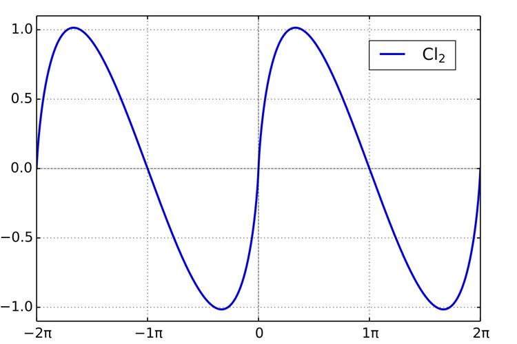
The Clausen function (of order 2) has simple zeros at all (integer) multiples of : π , since if : k ∈ Z is an integer, : sin k π = 0
Cl 2 ( m π ) = 0 , m = 0 , ± 1 , ± 2 , ± 3 , ⋯ It has maxim at : θ = π 3 + 2 m π [ m ∈ Z ]
Cl 2 ( π 3 + 2 m π ) = 1.01494160 … and minim at : θ = − π 3 + 2 m π [ m ∈ Z ]
Cl 2 ( − π 3 + 2 m π ) = − 1.01494160 … The following properties are immediate consequences of the series definition:
Cl 2 ( θ + 2 m π ) = Cl 2 ( θ ) Cl 2 ( − θ ) = − Cl 2 ( θ ) (Ref: See Lu and Perez, 1992, below for these results, although no proofs are given).
More generally, one defines the two generalized Clausen functions:
S z ( θ ) = ∑ k = 1 ∞ sin k θ k z C z ( θ ) = ∑ k = 1 ∞ cos k θ k z which are valid for complex z with Re z >1. The definition may be extended to all of the complex plane through analytic continuation.
When z is replaced with a non-negative integer, the Standard Clausen Functions are defined by the following Fourier series:
Cl 2 m + 2 ( θ ) = ∑ k = 1 ∞ sin k θ k 2 m + 2 Cl 2 m + 1 ( θ ) = ∑ k = 1 ∞ cos k θ k 2 m + 1 Sl 2 m + 2 ( θ ) = ∑ k = 1 ∞ cos k θ k 2 m + 2 Sl 2 m + 1 ( θ ) = ∑ k = 1 ∞ sin k θ k 2 m + 1 N.B. The SL-type Clausen functions have the alternative notation : Gl m ( θ ) and are sometimes referred to as the Glaisher–Clausen functions (after James Whitbread Lee Glaisher, hence the GL-notation).
The SL-type Clausen function are polynomials in θ , and are closely related to the Bernoulli polynomials. This connection is apparent from the Fourier series representations of the Bernoulli polynomials:
B 2 n − 1 ( x ) = 2 ( − 1 ) n ( 2 n − 1 ) ! ( 2 π ) 2 n − 1 ∑ k = 1 ∞ sin 2 π k x k 2 n − 1 . B 2 n ( x ) = 2 ( − 1 ) n − 1 ( 2 n ) ! ( 2 π ) 2 n ∑ k = 1 ∞ cos 2 π k x k 2 n . Setting x = θ / 2 π in the above, and then rearranging the terms gives the following closed form (polynomial) expressions:
Sl 2 m ( θ ) = ( − 1 ) m − 1 ( 2 π ) 2 m 2 ( 2 m ) ! B 2 m ( θ 2 π ) , Sl 2 m − 1 ( θ ) = ( − 1 ) m ( 2 π ) 2 m − 1 2 ( 2 m − 1 ) ! B 2 m − 1 ( θ 2 π ) , where the Bernoulli polynomials B n ( x ) are defined in terms of the Bernoulli numbers B n ≡ B n ( 0 ) by the relation:
B n ( x ) = ∑ j = 0 n ( n j ) B j x n − j . Explicit evaluations derived from the above include:
Sl 1 ( θ ) = π 2 − θ 2 , Sl 2 ( θ ) = π 2 6 − π θ 2 + θ 2 4 , Sl 3 ( θ ) = π 2 θ 6 − π θ 2 4 + θ 3 12 , Sl 4 ( θ ) = π 4 90 − π 2 θ 2 12 + π θ 3 12 − θ 4 48 . For : 0 < θ < π , the duplication formula can be proven directly from the Integral definition (see also Lu and Perez, 1992, below for the result – although no proof is given):
Cl 2 ( 2 θ ) = 2 Cl 2 ( θ ) − 2 Cl 2 ( π − θ ) Immediate consequences of the duplication formula, along with use of the special value : Cl 2 ( π 2 ) = G , include the relations:
Cl 2 ( π 4 ) − Cl 2 ( 3 π 4 ) = G 2 2 Cl 2 ( π 3 ) = 3 Cl 2 ( 2 π 3 ) For higher order Clausen functions, duplication formulae can be obtained from the one given above; simply replace θ with the dummy variable x , and integrate over the interval [ 0 , θ ] . Applying the same process repeatedly yields:
Cl 3 ( 2 θ ) = 4 Cl 3 ( θ ) + 4 Cl 3 ( π − θ ) Cl 4 ( 2 θ ) = 8 Cl 4 ( θ ) − 8 Cl 4 ( π − θ ) Cl 5 ( 2 θ ) = 16 Cl 5 ( θ ) + 16 Cl 5 ( π − θ ) Cl 6 ( 2 θ ) = 32 Cl 6 ( θ ) − 32 Cl 6 ( π − θ ) And more generally, upon induction on m , m ≥ 1
Cl m + 1 ( 2 θ ) = 2 m [ Cl m + 1 ( θ ) + ( − 1 ) m Cl m + 1 ( π − θ ) ] Use of the generalized duplication formula allows for an extension of the result for the Clausen function of order 2, involving Catalan's constant. For m ∈ Z ≥ 1
Cl 2 m ( π 2 ) = 2 2 m − 1 [ Cl 2 m ( p i 4 ) − Cl 2 m ( 3 π 4 ) ] = β ( 2 m ) Where β ( x ) is the Dirichlet beta function.
From the integral definition,
Cl 2 ( 2 θ ) = − ∫ 0 2 θ log | 2 sin x 2 | d x Apply the duplication formula for the sine function, : sin x = 2 sin x 2 cos x 2 to obtain
− ∫ 0 2 θ log | ( 2 sin x 4 ) ( 2 cos x 4 ) | d x = − ∫ 0 2 θ log | 2 sin x 4 | d x − ∫ 0 2 θ log | 2 cos x 4 | d x Apply the substitution x = 2 y , d x = 2 d y on both integrals:
− 2 ∫ 0 θ log | 2 sin x 2 | d x − 2 ∫ 0 θ log | 2 cos x 2 | d x = 2 Cl 2 ( θ ) − 2 ∫ 0 θ log | 2 cos x 2 | d x On that last integral, set y = π − x , x = π − y , d x = − d y , and use the trigonometric identity cos ( x − y ) = cos x cos y − sin x sin y to show that:
cos ( π − y 2 ) = sin y 2 ⟹ Cl 2 ( 2 θ ) = 2 Cl 2 ( θ ) − 2 ∫ 0 θ log | 2 cos x 2 | d x = 2 Cl 2 ( θ ) + 2 ∫ π π − θ log | 2 sin y 2 | d y = 2 Cl 2 ( θ ) − 2 Cl 2 ( π − θ ) + 2 Cl 2 ( π ) Cl 2 ( π ) = 0 Therefore,
Cl 2 ( 2 θ ) = 2 Cl 2 ( θ ) − 2 Cl 2 ( π − θ ) . ◻ Direct differentiation of the Fourier series expansions for the Clausen functions give:
d d θ Cl 2 m + 2 ( θ ) = d d θ ∑ k = 1 ∞ sin k θ k 2 m + 2 = ∑ k = 1 ∞ cos k θ k 2 m + 1 = Cl 2 m + 1 ( θ ) d d θ Cl 2 m + 1 ( θ ) = d d θ ∑ k = 1 ∞ cos k θ k 2 m + 1 = − ∑ k = 1 ∞ sin k θ k 2 m = − Cl 2 m ( θ ) d d θ Sl 2 m + 2 ( θ ) = d d θ ∑ k = 1 ∞ cos k θ k 2 m + 2 = − ∑ k = 1 ∞ sin k θ k 2 m + 1 = − Sl 2 m + 1 ( θ ) d d θ Sl 2 m + 1 ( θ ) = d d θ ∑ k = 1 ∞ sin k θ k 2 m + 1 = ∑ k = 1 ∞ cos k θ k 2 m = Sl 2 m ( θ ) By appealing to the First Fundamental Theorem Of Calculus, we also have:
d d θ Cl 2 ( θ ) = d d θ [ − ∫ 0 θ log | 2 sin x 2 | d x ] = − log | 2 sin θ 2 | = Cl 1 ( θ ) The inverse tangent integral is defined on the interval : 0 < z < 1 by
Ti 2 ( z ) = ∫ 0 z tan − 1 x x d x = ∑ k = 0 ∞ ( − 1 ) k z 2 k + 1 ( 2 k + 1 ) 2 It has the following closed form in terms of the Clausen Function:
Ti 2 ( tan θ ) = θ log ( tan θ ) + 1 2 Cl 2 ( 2 θ ) + 1 2 Cl 2 ( π − 2 θ ) From the integral definition of the inverse tangent integral, we have
Ti 2 ( tan θ ) = ∫ 0 tan θ tan − 1 x x d x Performing an integration by parts
∫ 0 tan θ tan − 1 x x d x = tan − 1 x log x | 0 tan θ − ∫ 0 tan θ log x 1 + x 2 d x = θ log tan θ − ∫ 0 tan θ log x 1 + x 2 d x Apply the substitution : x = tan y , y = tan − 1 x , d y = d x 1 + x 2 to obtain
θ log tan θ − ∫ 0 θ log ( tan y ) d y For that last integral, apply the transform : y = x / 2 , d y = d x / 2 to get
θ log tan θ − 1 2 ∫ 0 2 θ log ( tan x 2 ) d x = θ log tan θ − 1 2 ∫ 0 2 θ log ( sin ( x / 2 ) cos ( x / 2 ) ) d x = θ log tan θ − 1 2 ∫ 0 2 θ log ( 2 sin ( x / 2 ) 2 cos ( x / 2 ) ) d x = θ log tan θ − 1 2 ∫ 0 2 θ log ( 2 sin x 2 ) d x + 1 2 ∫ 0 2 θ log ( 2 cos x 2 ) d x = θ log tan θ + 1 2 Cl 2 ( 2 θ ) + 1 2 ∫ 0 2 θ log ( 2 cos x 2 ) d x . Finally, as with the proof of the Duplication formula, the substitution x = ( π − y ) reduces that last integral to
∫ 0 2 θ log ( 2 cos x 2 ) d x = Cl 2 ( π − 2 θ ) − Cl 2 ( π ) = Cl 2 ( π − 2 θ ) Thus
Ti 2 ( tan θ ) = θ log tan θ + 1 2 Cl 2 ( 2 θ ) + 1 2 Cl 2 ( π − 2 θ ) . ◻ For real : 0 < z < 1 , the Clausen function of second order can be expressed in terms of the Barnes G-function and (Euler) Gamma function:
Cl 2 ( 2 π z ) = 2 π log ( G ( 1 − z ) G ( 1 + z ) ) − 2 π z log ( sin π z π ) Or equivalently
Cl 2 ( 2 π z ) = 2 π log ( G ( 1 − z ) G ( z ) ) − 2 π log Γ ( z ) − 2 π log ( sin π z π ) Ref: See Adamchik, "Contributions to the Theory of the Barnes function", below.
The Clausen functions represent the real and imaginary parts of the polylogarithm, on the unit circle:
Cl 2 m ( θ ) = ℑ ( Li 2 m ( e i θ ) ) , m ∈ Z ≥ 1 Cl 2 m + 1 ( θ ) = ℜ ( Li 2 m + 1 ( e i θ ) ) , m ∈ Z ≥ 0 This is easily seen by appealing to the series definition of the polylogarithm.
Li n ( z ) = ∑ k = 1 ∞ z k k n ⟹ Li n ( e i θ ) = ∑ k = 1 ∞ ( e i θ ) k k n = ∑ k = 1 ∞ e i k θ k n By Euler's theorem,
e i θ = cos θ + i sin θ and by de Moivre's Theorem (De Moivre's formula)
( cos θ + i sin θ ) k = cos k θ + i sin k θ ⇒ Li n ( e i θ ) = ∑ k = 1 ∞ cos k θ k n + i ∑ k = 1 ∞ sin k θ k n Hence
Li 2 m ( e i θ ) = ∑ k = 1 ∞ cos k θ k 2 m + i ∑ k = 1 ∞ sin k θ k 2 m = Sl 2 m ( θ ) + i Cl 2 m ( θ ) Li 2 m + 1 ( e i θ ) = ∑ k = 1 ∞ cos k θ k 2 m + 1 + i ∑ k = 1 ∞ sin k θ k 2 m + 1 = Cl 2 m + 1 ( θ ) + i Sl 2 m + 1 ( θ ) The Clausen functions are intimately connected to the polygamma function. Indeed, it is possible to express Clausen functions as linear combinations of sine functions and polygamma functions. One such relation is shown here, and proven below:
Cl 2 m ( q π p ) = 1 ( 2 p ) 2 m ( 2 m − 1 ) ! ∑ j = 1 p sin ( q j π p ) [ ψ 2 m − 1 ( j 2 p ) + ( − 1 ) q ψ 2 m − 1 ( j + p 2 p ) ] Let p and q be positive integers, such that q / p is a rational number 0 < q / p < 1 , then, by the series definition for the higher order Clausen function (of even index):
Cl 2 m ( q π p ) = ∑ k = 1 ∞ sin ( k q π / p ) k 2 m We split this sum into exactly p-parts, so that the first series contains all, and only, those terms congruent to k p + 1 , the second series contains all terms congruent to k p + 2 , etc., up to the final p-th part, that contain all terms congruent to k p + p
Cl 2 m ( q π p ) = ∑ k = 0 ∞ sin [ ( k p + 1 ) q π p ] ( k p + 1 ) 2 m + ∑ k = 0 ∞ sin [ ( k p + 2 ) q π p ] ( k p + 2 ) 2 m + ∑ k = 0 ∞ sin [ ( k p + 3 ) q π p ] ( k p + 3 ) 2 m + ⋯ ⋯ + ∑ k = 0 ∞ sin [ ( k p + p − 2 ) q π p ] ( k p + p − 2 ) 2 m + ∑ k = 0 ∞ sin [ ( k p + p − 1 ) q π p ] ( k p + p − 1 ) 2 m + ∑ k = 0 ∞ sin [ ( k p + p ) q π p ] ( k p + p ) 2 m We can index these sums to form a double sum:
Cl 2 m ( q π p ) = ∑ j = 1 p { ∑ k = 0 ∞ sin [ ( k p + j ) q π p ] ( k p + j ) 2 m } = ∑ j = 1 p 1 p 2 m { ∑ k = 0 ∞ sin [ ( k p + j ) q π p ] ( k + ( j / p ) ) 2 m } Applying the addition formula for the sine function, sin ( x + y ) = sin x cos y + cos x sin y , the sine term in the numerator becomes:
sin [ ( k p + j ) q π p ] = sin ( k q π + q j π p ) = sin k q π cos q j π p + cos k q π sin q j π p sin m π ≡ 0 , cos m π ≡ ( − 1 ) m ⟺ m = 0 , ± 1 , ± 2 , ± 3 , … sin [ ( k p + j ) q π p ] = ( − 1 ) k q sin q j π p Consequently,
Cl 2 m ( q π p ) = ∑ j = 1 p 1 p 2 m sin ( q j π p ) { ∑ k = 0 ∞ ( − 1 ) k q ( k + ( j / p ) ) 2 m } To convert the inner sum in the double sum into a non-alternating sum, split in two in parts in exactly the same way as the earlier sum was split into p-parts:
∑ k = 0 ∞ ( − 1 ) k q ( k + ( j / p ) ) 2 m = ∑ k = 0 ∞ ( − 1 ) ( 2 k ) q ( ( 2 k ) + ( j / p ) ) 2 m + ∑ k = 0 ∞ ( − 1 ) ( 2 k + 1 ) q ( ( 2 k + 1 ) + ( j / p ) ) 2 m = ∑ k = 0 ∞ 1 ( 2 k + ( j / p ) ) 2 m + ( − 1 ) q ∑ k = 0 ∞ 1 ( 2 k + 1 + ( j / p ) ) 2 m = 1 2 p [ ∑ k = 0 ∞ 1 ( k + ( j / 2 p ) ) 2 m + ( − 1 ) q ∑ k = 0 ∞ 1 ( k + ( j + p 2 p ) ) 2 m ] For m ∈ Z ≥ 1 , the polygamma function has the series representation
ψ m ( z ) = ( − 1 ) m + 1 m ! ∑ k = 0 ∞ 1 ( k + z ) m + 1 So, in terms of the polygamma function, the previous inner sum becomes:
1 2 2 m ( 2 m − 1 ) ! [ ψ 2 m − 1 ( j 2 p ) + ( − 1 ) q ψ 2 m − 1 ( j + p 2 p ) ] Plugging this back into the double sum gives the desired result:
Cl 2 m ( q π p ) = 1 ( 2 p ) 2 m ( 2 m − 1 ) ! ∑ j = 1 p sin ( q j π p ) [ ψ 2 m − 1 ( j 2 p ) + ( − 1 ) q ψ 2 m − 1 ( j + p 2 p ) ] The generalized logsine integral is defined by:
L s n m ( θ ) = − ∫ 0 θ x m log n − m − 1 | 2 sin x 2 | d x In this generalized notation, the Clausen function can be expressed in the form:
Cl 2 ( θ ) = L s 2 0 ( θ ) Ernst Kummer and Rogers give the relation
Li 2 ( e i θ ) = ζ ( 2 ) − θ ( 2 π − θ ) / 4 + i Cl 2 ( θ ) valid for 0 ≤ θ ≤ 2 π .
The Lobachevsky function Λ or Л is essentially the same function with a change of variable:
Λ ( θ ) = − ∫ 0 θ log | 2 sin ( t ) | d t = Cl 2 ( 2 θ ) / 2 though the name "Lobachevsky function" is not quite historically accurate, as Lobachevsky's formulas for hyperbolic volume used the slightly different function
∫ 0 θ log | sec ( t ) | d t = Λ ( θ + π / 2 ) + θ log 2. For rational values of θ / π (that is, for θ / π = p / q for some integers p and q), the function sin ( n θ ) can be understood to represent a periodic orbit of an element in the cyclic group, and thus Cl s ( θ ) can be expressed as a simple sum involving the Hurwitz zeta function. This allows relations between certain Dirichlet L-functions to be easily computed.
A series acceleration for the Clausen function is given by
Cl 2 ( θ ) θ = 1 − log | θ | + ∑ n = 1 ∞ ζ ( 2 n ) n ( 2 n + 1 ) ( θ 2 π ) 2 n which holds for | θ | < 2 π . Here, ζ ( s ) is the Riemann zeta function. A more rapidly convergent form is given by
Cl 2 ( θ ) θ = 3 − log [ | θ | ( 1 − θ 2 4 π 2 ) ] − 2 π θ log ( 2 π + θ 2 π − θ ) + ∑ n = 1 ∞ ζ ( 2 n ) − 1 n ( 2 n + 1 ) ( θ 2 π ) n . Convergence is aided by the fact that ζ ( n ) − 1 approaches zero rapidly for large values of n. Both forms are obtainable through the types of resummation techniques used to obtain rational zeta series. (ref. Borwein, et al., 2000, below).
Some special values include
Cl 2 ( π 2 ) = G Cl 2 ( π 3 ) = 3 π log ( G ( 2 3 ) G ( 1 3 ) ) − 3 π log Γ ( 1 3 ) + π log ( 2 π 3 ) Cl 2 ( 2 π 3 ) = 2 π log ( G ( 2 3 ) G ( 1 3 ) ) − 2 π log Γ ( 1 3 ) + 2 π 3 log ( 2 π 3 ) Cl 2 ( π 4 ) = 2 π log ( G ( 7 8 ) G ( 1 8 ) ) − 2 π log Γ ( 1 8 ) + π 4 log ( 2 π 2 − 2 ) Cl 2 ( 3 π 4 ) = 2 π log ( G ( 5 8 ) G ( 3 8 ) ) − 2 π log Γ ( 3 8 ) + 3 π 4 log ( 2 π 2 + 2 ) Cl 2 ( π 6 ) = 2 π log ( G ( 11 12 ) G ( 1 12 ) ) − 2 π log Γ ( 1 12 ) + π 6 log ( 2 π 2 3 − 1 ) Cl 2 ( 5 π 6 ) = 2 π log ( G ( 7 12 ) G ( 5 12 ) ) − 2 π log Γ ( 5 12 ) + 5 π 6 log ( 2 π 2 3 + 1 ) Some special values for higher order Clausen functions include
Cl 2 m t ( 0 ) = Cl 2 m ( π ) = Cl 2 m ( 2 π ) = 0 Cl 2 m ( π 2 ) = β ( 2 m ) Cl 2 m + 1 ( 0 ) = Cl 2 m + 1 ( 2 π ) = ζ ( 2 m + 1 ) Cl 2 m + 1 ( π ) = − η ( 2 m + 1 ) = − ( 2 2 m − 1 2 2 m ) ζ ( 2 m + 1 ) Cl 2 m + 1 ( π 2 ) = − 1 2 2 m + 1 η ( 2 m + 1 ) = − ( 2 2 m − 1 2 4 m + 1 ) ζ ( 2 m + 1 ) where : G = β ( 2 ) is Catalan's constant, : β ( x ) is the Dirichlet beta function, : η ( x ) is the eta function (also called the alternating zeta function), and : ζ ( x ) is the Riemann zeta function.
β ( x ) = ∑ k = 0 ∞ ( − 1 ) k ( 2 k + 1 ) x The following integrals are easily proven from the series representations of the Clausen function:
∫ 0 θ Cl 2 m ( x ) d x = ζ ( 2 m + 1 ) − Cl 2 m + 1 ( θ ) ∫ 0 θ Cl 2 m + 1 ( x ) d x = Cl 2 m + 2 ( θ ) ∫ 0 θ Sl 2 m ( x ) d x = Sl 2 m + 1 ( θ ) ∫ 0 θ Sl 2 m + 1 ( x ) d x = ζ ( 2 m + 2 ) − Cl 2 m + 2 ( θ ) A large number of trigonometric and logarithmo-trigonometric integrals can be evaluated in terms of the Clausen function, and various common mathematical constants like G (Catalan's constant), log 2 , and the special cases of the zeta function, ζ ( 2 ) and ζ ( 3 ) .
The examples listed below follow directly from the integral representation of the Clausen function, and the proofs require little more than basic trigonometry, integration by parts, and occasional term-by-term integration of the Fourier series definitions of the Clausen functions.
∫ 0 θ log ( sin x ) d x = − 1 2 Cl 2 ( 2 θ ) − θ log 2 ∫ 0 θ log ( cos x ) d x = 1 2 Cl 2 ( π − 2 θ ) − θ log 2 ∫ 0 θ log ( tan x ) d x = − 1 2 Cl 2 ( 2 θ ) − 1 2 Cl 2 ( π − 2 θ ) ∫ 0 θ log ( 1 + cos x ) d x = 2 Cl 2 ( π − θ ) − θ log 2 ∫ 0 θ log ( 1 − cos x ) d x = − 2 Cl 2 ( θ ) − θ log 2 ∫ 0 θ log ( 1 + sin x ) d x = 2 G − 2 Cl 2 ( π 2 + θ ) − θ log 2 ∫ 0 θ log ( 1 − sin x ) d x = − 2 G + 2 Cl 2 ( π 2 − θ ) − θ log 2