CUSUM - Alchetron, The Free Social Encyclopedia

Originally proposed by E. S. Page Quality characteristic type Variables data Size of shift to detect ≤ 1.5σ		Rational subgroup size n = 1 Underlying distribution Normal distribution

Measurement type Cumulative sum of a quality characteristic

In statistical quality control, the CUSUM (or cumulative sum control chart) is a sequential analysis technique developed by E. S. Page of the University of Cambridge. It is typically used for monitoring change detection. CUSUM was announced in Biometrika, in 1954, a few years after the publication of Wald's SPRT algorithm.

Page referred to a "quality number" θ , by which he meant a parameter of the probability distribution; for example, the mean. He devised CUSUM as a method to determine changes in it, and proposed a criterion for deciding when to take corrective action. When the CUSUM method is applied to changes in mean, it can be used for step detection of a time series.

A few years later, George Alfred Barnard developed a visualization method, the V-mask chart, to detect both increases and decreases in θ .

Method

As its name implies, CUSUM involves the calculation of a cumulative sum (which is what makes it "sequential"). Samples from a process x n are assigned weights ω n , and summed as follows:

S 0 = 0 S n + 1 = max ( 0 , S n + x n − ω n )

When the value of S exceeds a certain threshold value, a change in value has been found. The above formula only detects changes in the positive direction. When negative changes need to be found as well, the min operation should be used instead of the max operation, and this time a change has been found when the value of S is below the (negative) value of the threshold value.

Page did not explicitly say that ω represents the likelihood function, but this is common usage.

Note that this differs from SPRT by always using zero function as the lower "holding barrier" rather than a lower "holding barrier". Also, CUSUM does not require the use of the likelihood function.

As a means of assessing CUSUM's performance, Page defined the average run length (A.R.L.) metric; "the expected number of articles sampled before action is taken." He further wrote:

When the quality of the output is satisfactory the A.R.L. is a measure of the expense incurred by the scheme when it gives false alarms, i.e., Type I errors (Neyman & Pearson, 1936). On the other hand, for constant poor quality the A.R.L. measures the delay and thus the amount of scrap produced before the rectifying action is taken, i.e., Type II errors.

Example

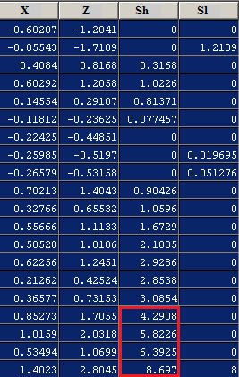
The following example shows 20 observations of a process with a mean value of X equal to 0 and a standard deviation of 0.5. It can be seen as the value of Z is never greater than 3, so other control charts should not be detected as a failure while using the Cusum 17 that shows the value of SH is greater than 4.

Variants

Cumulative observed-minus-expected plots are a related method.

References

CUSUM Wikipedia

(Text) CC BY-SA

Contents

Method

Example

Variants

References