
Data structure Array | ||
 | ||
Worst-case performance O ( n 2 ) {displaystyle O(n^{2})} Best-case performance Ω ( n + k ) {displaystyle Omega (n+k)} Average performance Θ ( n + k ) {displaystyle Theta (n+k)} Worst-case space complexity O ( n ⋅ k ) {displaystyle O(ncdot k)} | ||
Bucket sort, or bin sort, is a sorting algorithm that works by distributing the elements of an array into a number of buckets. Each bucket is then sorted individually, either using a different sorting algorithm, or by recursively applying the bucket sorting algorithm. It is a distribution sort, and is a cousin of radix sort in the most to least significant digit flavour. Bucket sort is a generalization of pigeonhole sort. Bucket sort can be implemented with comparisons and therefore can also be considered a comparison sort algorithm. The computational complexity estimates involve the number of buckets.
Contents
- Pseudocode
- Optimizations
- Generic bucket sort
- ProxmapSort
- Histogram sort
- Postmans sort
- Shuffle sort
- Comparison with other sorting algorithms
- References
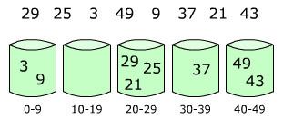
Bucket sort works as follows:
- Set up an array of initially empty "buckets".
- Scatter: Go over the original array, putting each object in its bucket.
- Sort each non-empty bucket.
- Gather: Visit the buckets in order and put all elements back into the original array.
Pseudocode
function bucketSort(array, n) is buckets ← new array of n empty lists for i = 0 to (length(array)-1) do insert array[i] into buckets[msbits(array[i], k)] for i = 0 to n - 1 do nextSort(buckets[i]); return the concatenation of buckets[0], ...., buckets[n-1]Here array is the array to be sorted and n is the number of buckets to use. The function msbits(x,k) returns the k most significant bits of x (floor(x/2^(size(x)-k))); different functions can be used to translate the range of elements in array to n buckets, such as translating the letters A–Z to 0–25 or returning the first character (0–255) for sorting strings. The function nextSort is a sorting function; using bucketSort itself as nextSort produces a relative of radix sort; in particular, the case n = 2 corresponds to quicksort (although potentially with poor pivot choices).
Note that for bucket sort to be
Optimizations
A common optimization is to put the unsorted elements of the buckets back in the original array first, then run insertion sort over the complete array; because insertion sort's runtime is based on how far each element is from its final position, the number of comparisons remains relatively small, and the memory hierarchy is better exploited by storing the list contiguously in memory.
Generic bucket sort
The most common variant of bucket sort operates on a list of n numeric inputs between zero and some maximum value M and divides the value range into n buckets each of size M/n. If each bucket is sorted using insertion sort, the sort can be shown to run in expected linear time (where the average is taken over all possible inputs). However, the performance of this sort degrades with clustering; if many values occur close together, they will all fall into a single bucket and be sorted slowly. This performance degradation is avoided in the original bucket sort algorithm by assuming that the input is generated by a random process that distributes elements uniformly over the interval [0,1). Since there are n uniformly distributed elements sorted in to n buckets the probable number of inputs in each bucket follows a binomial distribution with
ProxmapSort
Similar to generic bucket sort as described above, ProxmapSort works by dividing an array of keys into subarrays via the use of a "map key" function that preserves a partial ordering on the keys; as each key is added to its subarray, insertion sort is used to keep that subarray sorted, resulting in the entire array being in sorted order when ProxmapSort completes. ProxmapSort differs from bucket sorts in its use of the map key to place the data approximately where it belongs in sorted order, producing a "proxmap" — a proximity mapping — of the keys.
Histogram sort
Another variant of bucket sort known as histogram sort or counting sort adds an initial pass that counts the number of elements that will fall into each bucket using a count array. Using this information, the array values can be arranged into a sequence of buckets in-place by a sequence of exchanges, leaving no space overhead for bucket storage.
Postman's sort
The Postman's sort is a variant of bucket sort that takes advantage of a hierarchical structure of elements, typically described by a set of attributes. This is the algorithm used by letter-sorting machines in post offices: mail is sorted first between domestic and international; then by state, province or territory; then by destination post office; then by routes, etc. Since keys are not compared against each other, sorting time is O(cn), where c depends on the size of the key and number of buckets. This is similar to a radix sort that works "top down," or "most significant digit first."
Shuffle sort
The shuffle sort is a variant of bucket sort that begins by removing the first 1/8 of the n items to be sorted, sorts them recursively, and puts them in an array. This creates n/8 "buckets" to which the remaining 7/8 of the items are distributed. Each "bucket" is then sorted, and the "buckets" are concatenated into a sorted array.
Comparison with other sorting algorithms
Bucket sort can be seen as a generalization of counting sort; in fact, if each bucket has size 1 then bucket sort degenerates to counting sort. The variable bucket size of bucket sort allows it to use O(n) memory instead of O(M) memory, where M is the number of distinct values; in exchange, it gives up counting sort's O(n + M) worst-case behavior.
Bucket sort with two buckets is effectively a version of quicksort where the pivot value is always selected to be the middle value of the value range. While this choice is effective for uniformly distributed inputs, other means of choosing the pivot in quicksort such as randomly selected pivots make it more resistant to clustering in the input distribution.
The n-way mergesort algorithm also begins by distributing the list into n sublists and sorting each one; however, the sublists created by mergesort have overlapping value ranges and so cannot be recombined by simple concatenation as in bucket sort. Instead, they must be interleaved by a merge algorithm. However, this added expense is counterbalanced by the simpler scatter phase and the ability to ensure that each sublist is the same size, providing a good worst-case time bound.
Top-down radix sort can be seen as a special case of bucket sort where both the range of values and the number of buckets is constrained to be a power of two. Consequently, each bucket's size is also a power of two, and the procedure can be applied recursively. This approach can accelerate the scatter phase, since we only need to examine a prefix of the bit representation of each element to determine its bucket.