Broyden–Fletcher–Goldfarb–Shanno algorithm - Alchetron, the free social encyclopedia

In numerical optimization, the Broyden–Fletcher–Goldfarb–Shanno (BFGS) algorithm is an iterative method for solving unconstrained nonlinear optimization problems.

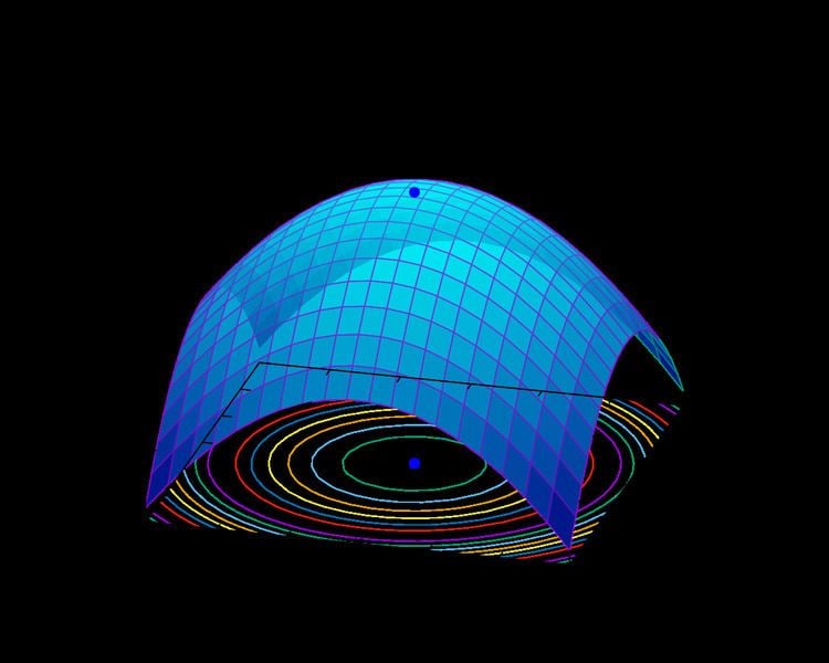
The BFGS method approximates Newton's method, a class of hill-climbing optimization techniques that seeks a stationary point of a (preferably twice continuously differentiable) function. For such problems, a necessary condition for optimality is that the gradient be zero. Newton's method and the BFGS methods are not guaranteed to converge unless the function has a quadratic Taylor expansion near an optimum. These methods use both the first and second derivatives of the function. However, BFGS has proven to have good performance even for non-smooth optimizations.

In quasi-Newton methods, the Hessian matrix of second derivatives doesn't need to be evaluated directly. Instead, the Hessian matrix is approximated using updates specified by gradient evaluations (or approximate gradient evaluations). Quasi-Newton methods are generalizations of the secant method to find the root of the first derivative for multidimensional problems. In multi-dimensional problems, the secant equation does not specify a unique solution, and quasi-Newton methods differ in how they constrain the solution. The BFGS method is one of the most popular members of this class. Also in common use is L-BFGS, which is a limited-memory version of BFGS that is particularly suited to problems with very large numbers of variables (e.g., >1000). The BFGS-B variant handles simple box constraints.

Rationale

The search direction p_k at stage k is given by the solution of the analogue of the Newton equation

B k p k = − ∇ f ( x k ) ,

where B k is an approximation to the Hessian matrix, which is updated iteratively at each stage, and ∇ f ( x k ) is the gradient of the function evaluated at x_k. A line search in the direction p_k is then used to find the next point x_k+1.

The quasi-Newton condition imposed on the update of B k is:

B k + 1 ( x k + 1 − x k ) = ∇ f ( x k + 1 ) − ∇ f ( x k ) .

Let y k = ∇ f ( x k + 1 ) − ∇ f ( x k ) and s k = x k + 1 − x k , then B k + 1 satisfies B k + 1 s k = y k which is the secant equation. The curvature condition s k ⊤ y k > 0 should be satisfied. If the function is not strongly convex, then the condition has to be enforced explicitly.

Instead of requiring the full Hessian matrix at the point x_k+1 to be computed as B_k+1, the approximate Hessian at stage k is updated by the addition of two matrices:

B k + 1 = B k + U k + V k .

Both U_k and V_k are symmetric rank-one matrices, but their sum is a rank-two update matrix. BFGS and DFP updating matrix both differ from its predecessor by a rank-two matrix. Another simpler rank-one method is known as Symmetric rank-one method which does not guarantee the positive definitiveness. In order to maintain the symmetry and positive definitiveness of B k + 1 , the update form can be chosen as: B k + 1 = B k + α u u ⊤ + β v v ⊤ . Imposing the secant condition, B k + 1 s k = y k . Choosing u = y k and v = B k s k , we can obtain:

α = 1 y k T s k . β = 1 s k T B k s k .

Finally, we substitute α and β into B k + 1 = B k + α u u ⊤ + β v v ⊤ and get the update equation of B k + 1 :

B k + 1 = B k + y k y k T y k T s k − B k s k s k T B k s k T B k s k .

Algorithm

From an initial guess x 0 and an approximate Hessian matrix B 0 the following steps are repeated as x k converges to the solution:

Obtain a direction p k by solving B k p k = − ∇ f ( x k ) .
Perform a line search to find an acceptable stepsize α k in the direction found in the first step, then update x k + 1 = x k + α k p k .
Set s k = α k p k .
y k = ∇ f ( x k + 1 ) − ∇ f ( x k ) .
B k + 1 = B k + y k y k T y k T s k − B k s k s k T B k s k T B k s k .

f ( x ) denotes the objective function to be minimized. Convergence can be checked by observing the norm of the gradient, | ∇ f ( x k ) | . Practically, B 0 can be initialized with B 0 = I , so that the first step will be equivalent to a gradient descent, but further steps are more and more refined by B k , the approximation to the Hessian.

The first step of the algorithm is carried out using the inverse of the matrix B k , which can be obtained efficiently by applying the Sherman–Morrison formula to the step 5 of the algorithm, giving

B k + 1 − 1 = ( I − s k y k T y k T s k ) B k − 1 ( I − y k s k T y k T s k ) + s k s k T y k T s k .

This can be computed efficiently without temporary matrices, recognizing that B k − 1 is symmetric, and that y k T B k − 1 y k and s k T y k are scalar, using an expansion such as

B k + 1 − 1 = B k − 1 + ( s k T y k + y k T B k − 1 y k ) ( s k s k T ) ( s k T y k ) 2 − B k − 1 y k s k T + s k y k T B k − 1 s k T y k .

In statistical estimation problems (such as maximum likelihood or Bayesian inference), credible intervals or confidence intervals for the solution can be estimated from the inverse of the final Hessian matrix. However, these quantities are technically defined by the true Hessian matrix, and the BFGS approximation may not converge to the true Hessian matrix.

Implementations

The GSL implements BFGS as gsl_multimin_fdfminimizer_vector_bfgs2. Ceres Solver implements both BFGS and L-BFGS.

In SciPy, the scipy.optimize.fmin_bfgs function implements BFGS. It is also possible to run BFGS using any of the L-BFGS algorithms by setting the parameter L to a very large number.

Octave uses BFGS with a double-dogleg approximation to the cubic line search.

In R, the BFGS algorithm (and the L-BFGS-B version that allows box constraints) is implemented as an option of the base function optim().

In the MATLAB Optimization Toolbox, the fminunc function uses BFGS with cubic line search when the problem size is set to "medium scale."

A high-precision arithmetic version of BFGS (pBFGS), implemented in C++ and integrated with the high-precision arithmetic package ARPREC is robust against numerical instability (e.g. round-off errors).

Another C++ implementation of BFGS (along with L-BFGS, L-BFGS-B, CG, and Newton's method) using Eigen (C++ library) are available on GitHub under the MIT License here.

BFGS and L-BFGS are also implemented in C as part of the open-source Gnu Regression, Econometrics and Time-series Library (gretl).

References

Broyden–Fletcher–Goldfarb–Shanno algorithm Wikipedia

(Text) CC BY-SA

Contents

Rationale

Algorithm

Implementations

References