Brooks–Iyengar algorithm

Background

The Brooks–Iyengar hybrid algorithm for distributed control in the presence of noisy data combines Byzantine agreement with sensor fusion. It bridges the gap between sensor fusion and Byzantine fault tolerance. This seminal algorithm unified these disparate fields for the first time. Essentially, it combines Dolev’s algorithm for approximate agreement with Mahaney and Schneider’s fast convergence algorithm (FCA). The algorithm assumes N processing elements (PEs), t of which are faulty and can behave maliciously. It takes as input either real values with inherent inaccuracy or noise (which can be unknown), or a real value with apriori defined uncertainty, or an interval. The output of the algorithm is a real value with an explicitly specified accuracy. The algorithm runs in O(NlogN) where N is the number of PEs: see Big O notation. It is possible to modify this algorithm to correspond to Crusader’s Convergence Algorithm (CCA), however, the bandwidth requirement will also increase. The algorithm has applications in distributed control, software reliability, High-performance computing, etc.

Algorithm

The Brooks–Iyengar algorithm is executed in every processing element (PE) of a distributed sensor network. Each PE exchanges their measured interval with all other PEs in the network. The "fused" measurement is a weighted average of the midpoints of the regions found. The concrete steps of Brooks–Iyengar algorithm are shown in this section. Each PE performs the algorithm separately:

Input:

The measurement sent by PE k to PE i is a closed interval [ l k , i , h k , i ] , 1 ≤ k ≤ N

Output:

The output of PE i includes a point estimate and an interval estimate

1. PE i receives measurements from all the other PEs.
2. Divide the union of collected measurements into mutually exclusive intervals based on the number of measurements that intersect, which is known as the weight of the interval.
3. Remove intervals with weight less than N − τ , where τ is the number of faulty PEs
4. If there are L intervals left, let A i denote the set of the remaining intervals. We have A i = { ( I 1 i , w 1 i ) , … , ( I L i , w L i ) } , where interval I l i = [ l I l i , h I l i ] and w l i is the weight associated with interval I l i . We also assume h I l i ≤ h I l + 1 i .
5. Calculate the point estimate v i ′ of PE i as v i ′ = ∑ l ( l I l i + h I l i ) ⋅ w l i 2 ∑ l w l i and the interval estimate is [ l I 1 i , h I L i ]

Example:

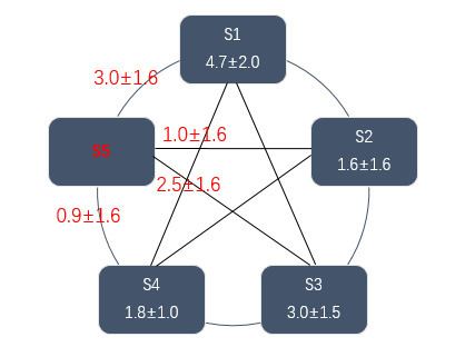
Consider an example of 5 PEs, in which PE 5 ( S 5 ) is sending wrong values to other PEs and they all exchange the values.

The values received by S 1 are in the next Table.

We draw a Weighted Region Diagram (WRD) of these intervals, then we can determine A 1 for PE 1 according to the Algorithm:

A 1 = { ( [ 1.5 , 2.7 ] , 4 ) , ( [ 2.7 , 2.8 ] , 5 ) , ( [ 2.8 , 3.2 ] , 4 ) }

which consists of intervals where at least 4(= N − τ = 5−1) measurements intersect. The output of PE 1 is equal to

4 ∗ 1.5 + 2.7 2 + 5 ∗ 2.7 + 2.8 2 + 4 ∗ 2.8 + 3.2 2 13 = 2.625

and the interval estimate is [ 1.5 , 3.2 ]

Similar, we could obtain all the inputs and results of the 5 PEs:

Related Algorithms

1982 Byzantine Problem: The Byzantine General Problem as an extension of Two Generals' Problem could be viewed as a binary problem.

1983 Approximate Consensus: The method removes some values from the set consists of scalars to tolerant faulty inputs.

1985 In-exact Consensus: The method also uses scalar as the input.

1996 Brooks-Iyengar Algorithm: The method is based on intervals.

2013 Byzantine Vector Consensus: The method uses vectors as the input.

2013 Multidimensional Agreement: The method also use vectors as the input while the measure of distance is different.

We could use Approximate Consensus (scalar-based), Brooks-Iyengar Algorithm (interval-based) and Byzantine Vector Consensus (vector-based) to deal with interval inputs, and the paper proved that Brooks–Iyengar algorithm is the best here.

Application

Brooks–Iyengar algorithm is a seminal work and a major milestone in distributed sensing, and could be used as a fault tolerant solution for many redundancy scenarios. Also, it is easy to implement and embed in any networking systems.

In 1996, the algorithm was used in MINIX to provide more accuracy and precision, which leads to the development of the first version of RT-Linux.

In 2000, the algorithm was also central to the DARPA SensIT program’s distributed tracking program. Acoustic, seismic and motion detection readings from multiple sensors are combined and fed into a distributed tracking system. Besides, it was used to combine heterogeneous sensor feeds in the application fielded by BBN Technologies, BAE systems, Penn State Applied Research Lab(ARL), and USC/ISI.

Besides, the Thales Group, an UK Defense Manufacturer, used this work in its Global Operational Analysis Laboratory. It is applied to Raytheon’s programs where many systems need extract reliable data from unreliable sensor network, this exempts the increasing investment in improving sensor reliability. Also, the research in developing this algorithm results in the tools used by the US Nav in its maritime domain awareness software.

In education, Brooks–Iyengar algorithm has been widely used in teaching classes such as University of Wisconsin, Purdue, Georgia Tech, Clemson University, University of Maryland, etc.

In addition to the area of sensor network, other fields such as time-triggered architecture, safety of cyber-physical systems, data fusion, robot convergence, high-performance computing, software/hardware reliability, ensemble learning in artificial intelligence systems could also benefit from Brooks–Iyengar algorithm.

Algorithm characteristics