Bresenham's line algorithm

History

Bresenham's line algorithm is named after Jack Elton Bresenham who developed it in 1962 at IBM. In 2001 Bresenham wrote:

I was working in the computation lab at IBM's San Jose development lab. A Calcomp plotter had been attached to an IBM 1401 via the 1407 typewriter console. [The algorithm] was in production use by summer 1962, possibly a month or so earlier. Programs in those days were freely exchanged among corporations so Calcomp (Jim Newland and Calvin Hefte) had copies. When I returned to Stanford in Fall 1962, I put a copy in the Stanford comp center library. A description of the line drawing routine was accepted for presentation at the 1963 ACM national convention in Denver, Colorado. It was a year in which no proceedings were published, only the agenda of speakers and topics in an issue of Communications of the ACM. A person from the IBM Systems Journal asked me after I made my presentation if they could publish the paper. I happily agreed, and they printed it in 1965.

Bresenham's algorithm was later extended to produce circles, the resulting algorithm being sometimes known as either Bresenham's circle algorithm or midpoint circle algorithm.

Method

The following conventions will be used:

the top-left is (0,0) such that pixel coordinates increase in the right and down directions (e.g. that the pixel at (7,4) is directly above the pixel at (7,5)), and

that the pixel centers have integer coordinates.

The endpoints of the line are the pixels at ( x 0 , y 0 ) and ( x 1 , y 1 ) , where the first coordinate of the pair is the column and the second is the row.

The algorithm will be initially presented only for the octant in which the segment goes down and to the right ( x 0 ≤ x 1 and y 0 ≤ y 1 ), and its horizontal projection x 1 − x 0 is longer than the vertical projection y 1 − y 0 (the line has a negative slope whose absolute value is less than 1). In this octant, for each column x between x 0 and x 1 , there is exactly one row y (computed by the algorithm) containing a pixel of the line, while each row between y 0 and y 1 may contain multiple rasterized pixels.

Bresenham's algorithm chooses the integer y corresponding to the pixel center that is closest to the ideal (fractional) y for the same x; on successive columns y can remain the same or increase by 1. The general equation of the line through the endpoints is given by:

y − y 0 y 1 − y 0 = x − x 0 x 1 − x 0 .

Since we know the column, x, the pixel's row, y, is given by rounding this quantity to the nearest integer:

y = y 1 − y 0 x 1 − x 0 ( x − x 0 ) + y 0 .

The slope ( y 1 − y 0 ) / ( x 1 − x 0 ) depends on the endpoint coordinates only and can be precomputed, and the ideal y for successive integer values of x can be computed starting from y 0 and repeatedly adding the slope.

In practice, the algorithm does not keep track of the y coordinate, which increases by m = ∆y/∆x each time the x increases by one; it keeps an error bound at each stage, which represents the negative of the distance from (a) the point where the line exits the pixel to (b) the top edge of the pixel. This value is first set to m − 0.5 (due to using the pixel's center coordinates), and is incremented by m each time the x coordinate is incremented by one. If error becomes greater than 0.5, we know that the line has moved upwards one pixel, and that we must increment our y coordinate and readjust the error to represent the distance from the top of the new pixel – which is done by subtracting one from error.

In the following pseudocode sample plot(x,y) plots the pixel centered at coordinates (x,y) and abs returns absolute value:

function line(x0, y0, x1, y1) real deltax := x1 - x0 real deltay := y1 - y0 real deltaerr := abs(deltay / deltax) // Assume deltax != 0 (line is not vertical), // note that this division needs to be done in a way that preserves the fractional part real error := deltaerr - 0.5 int y := y0 for x from x0 to x1 plot(x,y) error := error + deltaerr if error ≥ 0.5 then y := y + 1 error := error - 1.0

Derivation

To derive Bresenham's algorithm, two steps must be taken. The first step is transforming the equation of a line from the typical slope-intercept form into something different; and then using this new equation for a line to draw a line based on the idea of accumulation of error.

Line equation

The slope-intercept form of a line is written as

y = f ( x ) = m x + b

where m is the slope and b is the y-intercept. This is a function of only x and it would be useful to make this equation written as a function of both x and y. Using algebraic manipulation and recognition that the slope is the "rise over run" or Δ y / Δ x then

y = m x + b y = ( Δ y ) ( Δ x ) x + b ( Δ x ) y = ( Δ y ) x + ( Δ x ) b 0 = ( Δ y ) x − ( Δ x ) y + ( Δ x ) b

Letting this last equation be a function of x and y then it can be written as

f ( x , y ) = 0 = A x + B y + C

where the constants are

A = Δ y

B = − Δ x

C = ( Δ x ) b

The line is then defined for some constants A, B, and C anywhere f ( x , y ) = 0 . For any ( x , y ) not on the line then f ( x , y ) ≠ 0 . It should be noted that everything about this form involves only integers if x and y are integers since the constants are necessarily integers.

As an example, the line y = 1 2 x + 1 then this could be written as f ( x , y ) = x − 2 y + 2 . The point (2,2) is on the line

f ( 2 , 2 ) = x − 2 y + 2 = ( 2 ) − 2 ( 2 ) + 2 = 2 − 4 + 2 = 0

and the point (2,3) is not on the line

f ( 2 , 3 ) = ( 2 ) − 2 ( 3 ) + 2 = 2 − 6 + 2 = − 2

and neither is the point (2,1)

f ( 2 , 1 ) = ( 2 ) − 2 ( 1 ) + 2 = 2 − 2 + 2 = 2

Notice that the points (2,1) and (2,3) are on opposite sides of the line and f(x,y) evaluates to positive or negative. A line splits a plane into halves and the half-plane that has a negative f(x,y) can be called the negative half-plane, and the other half can called the positive half-plane. This observation is very important in the remainder of the derivation.

Algorithm

Clearly, the starting point is on the line

f ( x 0 , y 0 ) = 0

only because the line is defined to start and end on integer coordinates (though it is entirely reasonable to want to draw a line with non-integer end points).

Keeping in mind that the slope is less-than-or-equal-to zero, the problem now presents itself as to whether the next point should be at ( x 0 + 1 , y 0 ) or ( x 0 + 1 , y 0 + 1 ) . Perhaps intuitively, the point should be chosen based upon which is closer to the line at x 0 + 1 . If it is closer to the former then include the former point on the line, if the latter then the latter. To answer this, evaluate the line function at the midpoint between these two points:

f ( x 0 + 1 , y 0 + 1 / 2 )

If the value of this is positive then the ideal line is below the midpoint and closer to the candidate point ( x 0 + 1 , y 0 + 1 ) ; in effect the y coordinate has advanced. Otherwise, the ideal line passes through or above the midpoint, and the y coordinate has not advanced; in this case choose the point ( x 0 + 1 , y 0 ) . This observation is crucial to understand! The value of the line function at this midpoint is the sole determinant of which point should be chosen.

The image to the right shows the blue point (2,2) chosen to be on the line with two candidate points in green (3,2) and (3,3). The black point (3, 2.5) is the midpoint between the two candidate points.

Algorithm for integer arithmetic

Alternatively, the difference between points can be used instead of evaluating f(x,y) at midpoints. This alternative method allows for integer-only arithmetic, which is generally faster than using floating-point arithmetic. To derive the alternative method, define the difference to be as follows:

D = f ( x 0 + 1 , y 0 + 1 / 2 ) − f ( x 0 , y 0 )

For the first decision, this formulation is equivalent to the midpoint method since f ( x 0 , y 0 ) = 0 at the starting point. Simplifying this expression yields:

D = [ A ( x 0 + 1 ) + B ( y 0 + 1 2 ) + C ] − [ A x 0 + B y 0 + C ] = [ A x 0 + B y 0 + C + A + 1 2 B ] − [ A x 0 + B y 0 + C ] = A + 1 2 B

Just as with the midpoint method, if D is positive, then choose ( x 0 + 1 , y 0 + 1 ) , otherwise choose ( x 0 + 1 , y 0 ) .

The decision for the second point can be written as

f ( x 0 + 2 , y 0 + 1 / 2 ) − f ( x 0 + 1 , y 0 + 1 / 2 ) = A = Δ y f ( x 0 + 2 , y 0 + 3 / 2 ) − f ( x 0 + 1 , y 0 + 1 / 2 ) = A + B = Δ y − Δ x

If the difference is positive then ( x 0 + 2 , y 0 + 1 ) is chosen, otherwise ( x 0 + 2 , y 0 ) . This decision can be generalized by accumulating the error.

All of the derivation for the algorithm is done. One performance issue is the 1/2 factor in the initial value of D. Since all of this is about the sign of the accumulated difference, then everything can be multiplied by 2 with no consequence.

This results in an algorithm that uses only integer arithmetic.

plotLine(x0,y0, x1,y1) dx = x1 - x0 dy = y1 - y0 D = 2*dy - dx y = y0 for x from x0 to x1 plot(x,y) if D > 0 y = y + 1 D = D - 2*dx end if D = D + 2*dy

Running this algorithm for f ( x , y ) = x − 2 y + 2 from (0,1) to (6,4) yields the following differences with dx=6 and dy=3:

D=2*3-6=0

Loop from 0 to 6

x=0: plot(0,1), D≤0: D=0+3=3

x=1: plot(1,1), D>0: D=3-6=-3, y=1+1=2, D=-3+3=0

x=2: plot(2,2), D≤0: D=0+3=3

x=3: plot(3,2), D>0: D=3-6=-3, y=2+1=3, D=-3+3=0

x=4: plot(4,3), D≤0: D=0+3=3

x=5: plot(5,3), D>0: D=3-6=-3, y=3+1=4, D=-3+3=0

x=6: plot(6,4), D≤0: D=0+3=3

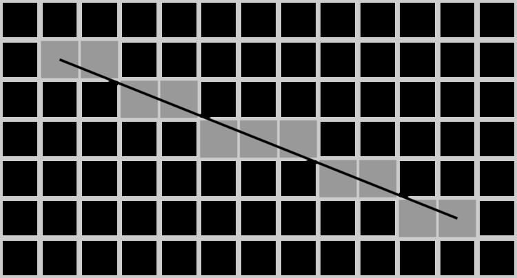
The result of this plot is shown to the right. The plotting can be viewed by plotting at the intersection of lines (blue circles) or filling in pixel boxes (yellow squares). Regardless, the plotting is the same.

All cases

However, as mentioned above this is only for the first octant. This means there are eight possible cases to consider. The simplest way to extend the same algorithm, if implemented in hardware, is to flip the co-ordinate system on the input and output of the single-octant drawer.

// Function to apply on the input function switchToOctantZeroFrom(octant, x, y) switch(octant) case 0: return (x, y) case 1: return (y, x) case 2: return (y, -x) case 3: return (-x, y) case 4: return (-x, -y) case 5: return (-y, -x) case 6: return (-y, x) case 7: return (x, -y) // Function to apply on the output (almost the same but cases 2 and 6 are swapped) function switchFromOctantZeroTo(octant, x, y) switch(octant) case 0: return (x, y) case 1: return (y, x) case 2: return (-y, x) case 3: return (-x, y) case 4: return (-x, -y) case 5: return (-y, -x) case 6: return (y, -x) case 7: return (x, -y) Octants: 2|1/ 3|/0 ---+--- 4/|7 /5|6

Similar algorithms

The Bresenham algorithm can be interpreted as slightly modified digital differential analyzer (using 0.5 as error threshold instead of 0, which is required for non-overlapping polygon rasterizing).

The principle of using an incremental error in place of division operations has other applications in graphics. It is possible to use this technique to calculate the U,V co-ordinates during raster scan of texture mapped polygons. The voxel heightmap software-rendering engines seen in some PC games also used this principle.

Bresenham also published a Run-Slice (as opposed to the Run-Length) computational algorithm.

An extension to the algorithm that handles thick lines was created by Alan Murphy at IBM.