Bland–Altman plot

Agreement vs correlation

Bland and Altman make the point that any two methods that are designed to measure the same parameter (or property) should have good correlation when a set of samples are chosen such that the property to be determined varies considerably. A high correlation for any two methods designed to measure the same property could thus in itself just be a sign that one has chosen a widespread sample. A high correlation does not necessarily imply that there is good agreement between the two methods.

How to construct a Bland–Altman plot

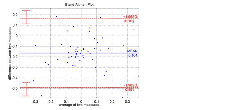
Consider a set of n samples (for example, objects of unknown volume). Both assays (for example, different methods of volume measurement) are performed on each sample, resulting in 2n data points. Each of the n samples is then represented on the graph by assigning the mean of the two measurements as the abscissa (x-axis) value, and the difference between the two values as the ordinate (y-axis) value.

Hence, the Cartesian coordinates of a given sample S with values of S 1 and S 2 determined by the two assays is

For comparing the dissimilarities between the two sets of samples independently from their mean values, it is more appropriate to look at the ratio of the pairs of measurements. Log transformation (base 2) of the measurements before the analysis will enable the standard approach to be used; hence the plot will be given by the following equation:

This version of the plot is used in MA plot.

Application

One primary application of the Bland–Altman plot is to compare two clinical measurements that each provide some errors in their measure. It can also be used to compare a new measurement technique or method with a gold standard, as even a gold standard does not - and should not - imply it to be without error. See Analyse-it, MedCalc, NCSS, GraphPad Prism, R, or StatsDirect for software providing Bland–Altman plots.

Bland and Altman plots are extensively used to evaluate the agreement among two different instruments or two measurements techniques. Bland and Altman plots allow identification of any systematic difference between the measurements (i.e., fixed bias) or possible outliers. The mean difference is the estimated bias, and the SD of the differences measures the random fluctuations around this mean. If the mean value of the difference differs significantly from 0 on the basis of a 1-sample t-test, this indicates the presence of fixed bias. If there is a consistent bias, it can be adjusted for by subtracting the mean difference from the new method. It is common to compute 95% limits of agreement for each comparison (average difference ± 1.96 standard deviation of the difference), which tells us how far apart measurements by 2 methods were more likely to be for most individuals. If the differences within mean ± 1.96 SD are not clinically important, the two methods may be used interchangeably. The 95% limits of agreement can be unreliable estimates of the population parameters especially for small sample sizes so, when comparing methods or assessing repeatability, it is important to calculate confidence intervals for 95% limits of agreement. This can be done by Bland and Altman's approximate method or by more precise methods.

Bland and Altman plots were also used to investigate any possible relationship of the discrepancies between the measurements and the true value (i.e., proportional bias). The existence of proportional bias indicates that the methods do not agree equally through the range of measurements (i.e., the limits of agreement will depend on the actual measurement). To evaluate this relationship formally, the difference between the methods should be regressed on the average of the 2 methods. When a relationship between the differences and the true value was identified (i.e., a significant slope of the regression line), regression-based 95% limits of agreement should be provided.