
 | ||
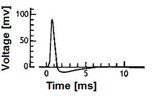
A biological neuron model, also known as a spiking neuron model, is a mathematical description of the properties of certain cells in the nervous system that generate sharp electrical potentials across their cell membrane, roughly one millisecond in duration, as shown in Fig. 1. Spiking neurons are known to be a major signaling unit of the nervous system, and for this reason characterizing their operation is of great importance. It is worth noting that not all the cells of the nervous system produce the type of spike that define the scope of the spiking neuron models. For example, cochlear hair cells, retinal receptor cells, and retinal bipolar cells do not spike. Furthermore, many cells in the nervous system are not classified as neurons but instead are classified as glia.
Contents
- Electrical inputoutput membrane voltage models
- Integrate and fire
- HodgkinHuxley model
- Leaky integrate and fire
- Fractional Order Leaky integrate and fire
- Galves Lcherbach
- Exponential integrate and fire
- FitzHughNagumo
- MorrisLecar
- HindmarshRose
- Cable theory
- Compartmental models
- Natural input stimulus neuron models
- The non homogeneous Poisson process model Siebert
- The two state Markov model Nossenson Messer
- Non Markovian models
- Pharmacological input stimulus neuron models
- Synaptic transmission Koch Segev
- Applications
- Electrical retinal prosthesis
- Neurotransmitter based retinal prosthesis
- Artificial limb control and sensation
- Conjecture 1 Relation between artificial and biological neuron models
- Conjecture 3 The neurotransmitter based energy detection scheme
- General comments regarding the modern perspective of scientific and engineering models
- References
Ultimately, biological neuron models aim to explain the mechanisms underlying the operation of the nervous system for the purpose of restoring lost control capabilities such as perception (e.g. deafness or blindness), motor movement decision making, and continuous limb control. In that sense, biological neural models differ from artificial neuron models that do not presume to predict the outcomes of experiments involving the biological neural tissue (although artificial neuron models are also concerned with execution of perception and estimation tasks). Accordingly, an important aspect of biological neuron models is experimental validation, and the use of physical units to describe the experimental procedure associated with the model predictions.
Neuron models can be divided into two categories according to the physical units of the interface of the model. Each category could be further divided according to the abstraction/detail level:
- Electrical input–output membrane voltage models – These models produce a prediction for membrane output voltage as function of electrical stimulation at the input stage (either voltage or current). The various models in this category differ in the exact functional relationship between the input current and the output voltage and in the level of details. Some models in this category are black box models and distinguish only between two measured voltage levels: the presence of a spike (also known as "action potential") or a quiescent state. Other models are more detailed and account for sub-cellular processes.
- Natural or pharmacological input neuron models – The models in this category connect between the input stimulus which can be either pharmacological or natural, to the probability of a spike event. The input stage of these models is not electrical, but rather has either pharmacological (chemical) concentration units, or physical units that characterize an external stimulus such as light, sound or other forms of physical pressure. Furthermore, the output stage represents the probability of a spike event and not an electrical voltage. Typically, this output probability is normalized (divided by) a time constant, and the resulting normalized probability is called the "firing rate" and has units of Hertz. The probabilistic description taken by the models in this category was inspired from laboratory experiments involving either natural or pharmacological stimulation which exhibit variability in the resulting spike pattern. Nevertheless, when averaging these experimental results across several trials, a clear pattern is often revealed.
Although it is not unusual in science and engineering to have several descriptive models for different abstraction/detail levels, the number of different, sometimes contradicting, biological neuron models is exceptionally high. This situation is partly the result of the many different experimental settings, and the difficulty to separate the intrinsic properties of a single neuron from measurements effects and interactions of many cells (network effects). To accelerate the convergence to a unified theory, we list several models in each category, and where applicable, also references to supporting experiments.
Electrical input–output membrane voltage models
The models in this category describe the relationship between neuronal membrane currents at the input stage, and membrane voltage at the output stage. The most extensive experimental inquiry in this category of models was made by Hodgkin–Huxley in the early 1950s using an experimental setup that punctured the cell membrane and allowed to force a specific membrane voltage/current.
Most modern electrical neural interfaces apply extra-cellular electrical stimulation to avoid membrane puncturing which can lead to cell death and tissue damage. Hence, it is not clear to what extent the electrical neuron models hold for extra-cellular stimulation (see e.g.).
Integrate-and-fire
One of the earliest models of a neuron was first investigated in 1907 by Louis Lapicque. A neuron is represented in time by
which is just the time derivative of the law of capacitance, Q = CV. When an input current is applied, the membrane voltage increases with time until it reaches a constant threshold Vth, at which point a delta function spike occurs and the voltage is reset to its resting potential, after which the model continues to run. The firing frequency of the model thus increases linearly without bound as input current increases.
The model can be made more accurate by introducing a refractory period tref that limits the firing frequency of a neuron by preventing it from firing during that period. Through some calculus involving a Fourier transform, the firing frequency as a function of a constant input current thus looks like
A remaining shortcoming of this model is that it implements no time-dependent memory. If the model receives a below-threshold signal at some time, it will retain that voltage boost forever until it fires again. This characteristic is clearly not in line with observed neuronal behavior.
Hodgkin–Huxley model
The Hodgkin–Huxley model (H&H model) is a model of the relationship between ion currents crossing the neuronal cell membrane and the membrane voltage. The model is based on experiments that allowed to force membrane voltage using an intra-cellular pipette. This model is based on the concept of membrane ion channels and relies on data from the squid giant axon. Hodgkin-Huxley was awarded the 1963 Nobel Prize in Physiology or Medicine for this model.
We note as before our voltage-current relationship, this time generalized to include multiple voltage-dependent currents:
Each current is given by Ohm's Law as
where g(t,V) is the conductance, or inverse resistance, which can be expanded in terms of its constant average ḡ and the activation and inactivation fractions m and h, respectively, that determine how many ions can flow through available membrane channels. This expansion is given by
and our fractions follow the first-order kinetics
with similar dynamics for h, where we can use either τ and m∞ or α and β to define our gate fractions.
With such a form, all that remains is to individually investigate each current one wants to include. Typically, these include inward Ca2+ and Na+ input currents and several varieties of K+ outward currents, including a "leak" current.
The end result can be at the small end 20 parameters which one must estimate or measure for an accurate model, and for complex systems of neurons not easily tractable by computer. Careful simplifications of the Hodgkin–Huxley model are therefore needed.
Leaky integrate-and-fire
In the leaky integrate-and-fire model, the memory problem is solved by adding a "leak" term to the membrane potential, reflecting the diffusion of ions that occurs through the membrane when some equilibrium is not reached in the cell. The model looks like
where Rm is the membrane resistance, as we find it is not a perfect insulator as assumed previously. This forces the input current to exceed some threshold Ith = Vth / Rm in order to cause the cell to fire, else it will simply leak out any change in potential. The firing frequency thus looks like
which converges for large input currents to the previous leak-free model with refractory period.
Fractional-Order Leaky integrate-and-fire
Recent advances in computational and theoretical fractional calculus lead to a new form of model, called Fractional-Order Leaky integrate-and-fire developed by Teka et al. The great advantage of this model is that it can capture and integrate all the past activities and can reproduce the time dependent spiking adaptations observed on pyramidal neurons. The model has the following form more details can be found in
Galves-Löcherbach
The Galves-Löcherbach model is a specific development of the leaky integrate-and-fire model. It is inherently stochastic. It was developed by mathematicians Antonio Galves and Eva Löcherbach. Given the model specifications, the probability that a given neuron
where
Exponential integrate-and-fire
In the Exponential Integrate-and-Fire, spike generation is exponential, following the equation:
where
FitzHugh–Nagumo
Sweeping simplifications to Hodgkin–Huxley were introduced by FitzHugh and Nagumo in 1961 and 1962. Seeking to describe "regenerative self-excitation" by a nonlinear positive-feedback membrane voltage and recovery by a linear negative-feedback gate voltage, they developed the model described by
where we again have a membrane-like voltage and input current with a slower general gate voltage w and experimentally-determined parameters a = -0.7, b = 0.8, τ = 1/0.08. Although not clearly derivable from biology, the model allows for a simplified, immediately available dynamic, without being a trivial simplification.
Morris–Lecar
In 1981 Morris and Lecar combined Hodgkin–Huxley and FitzHugh–Nagumo into a voltage-gated calcium channel model with a delayed-rectifier potassium channel, represented by
where
Hindmarsh–Rose
Building upon the FitzHugh–Nagumo model, Hindmarsh and Rose proposed in 1984 a model of neuronal activity described by three coupled first order differential equations:
with r2 = x2 + y2 + z2, and r ≈ 10−2 so that the z variable only changes very slowly. This extra mathematical complexity allows a great variety of dynamic behaviors for the membrane potential, described by the x variable of the model, which include chaotic dynamics. This makes the Hindmarsh–Rose neuron model very useful, because being still simple, allows a good qualitative description of the many different patterns of the action potential observed in experiments.
Cable theory
Cable theory describes the dendritic arbor as a cylindrical structure undergoing a regular pattern of bifurcation, like branches in a tree. For a single cylinder or an entire tree, the input conductance at the base (where the tree meets the cell body, or any such boundary) is defined as
where L is the electrotonic length of the cylinder which depends on its length, diameter, and resistance. A simple recursive algorithm scales linearly with the number of branches and can be used to calculate the effective conductance of the tree. This is given by
where AD = πld is the total surface area of the tree of total length l, and LD is its total electrotonic length. For an entire neuron in which the cell body conductance is GS and the membrane conductance per unit area is Gmd = Gm / A, we find the total neuron conductance GN for n dendrite trees by adding up all tree and soma conductances, given by
where we can find the general correction factor Fdga experimentally by noting GD = GmdADFdga.
Compartmental models
The cable model makes a number of simplifications to give closed analytic results, namely that the dendritic arbor must branch in diminishing pairs in a fixed pattern. A compartmental model allows for any desired tree topology with arbitrary branches and lengths, but makes simplifications in the interactions between branches to compensate. Thus, the two models give complementary results, neither of which is necessarily more accurate.
Each individual piece, or compartment, of a dendrite is modeled by a straight cylinder of arbitrary length l and diameter d which connects with fixed resistance to any number of branching cylinders. We define the conductance ratio of the ith cylinder as Bi = Gi / G∞, where
where the last equation deals with parents and daughters at branches, and
An example of a compartmental model of a neuron, with an algorithm to reduce the number of compartments (increase the computational speed) and yet retain the salient electrical characteristics, can be found in.
Natural input stimulus neuron models
The models in this category were derived following experiments involving natural stimulation such as light, sound, touch, or odor. In these experiments, the spike pattern resulting from each stimulus presentation varies from trial to trial, but the averaged response from several trials often converges to a clear pattern. Consequently, the models in this category generate a probabilistic relationship between the input stimulus to spike occurrences.
The non-homogeneous Poisson process model (Siebert)
Siebert modeled the neuron spike firing pattern using a non-homogeneous Poisson process model, following experiments involving the auditory system. According to Siebert, the probability of a spiking event at the time interval
Siebert considered several functions as
The main advantage of Siebert's model is its simplicity. The shortcomings of the model is its inability to reflect properly the following phenomena:
These shortcoming are addressed by the two state Markov Model.
The two state Markov model (Nossenson & Messer)
The spiking neuron model by Nossenson & Messer produces the probability of the neuron to fire a spike as a function of either an external or pharmacological stimulus. The model consists of a cascade of a receptor layer model and a spiking neuron model, as shown in Fig 4. The connection between the external stimulus to the spiking probability is made in two steps: First, a receptor cell model translates the raw external stimulus to neurotransmitter concentration, then, a spiking neuron model connects between neurotransmitter concentration to the firing rate (spiking probability). Thus, the spiking neuron model by itself depends on neurotransmitter concentration at the input stage.
An important feature of this model is the prediction for neurons firing rate pattern which captures, using a low number of free parameters, the characteristic edge emphasized response of neurons to a stimulus pulse, as shown in Fig. 5. The firing rate is identified both as a normalized probability for neural spike firing, and as a quantity proportional to the current of neurotransmitters released by the cell. The expression for the firing rate takes the following form:
where,
P0 could be generally calculated recursively using Euler method, but in the case of a pulse of stimulus it yields a simple closed form expression.
Other predictions by this model include:
1) The averaged Evoked Response Potential (ERP) due to population of many neurons in unfiltered measurements resembles the firing rate.
2) The voltage variance of activity due to multiple neuron activity resembles the firing rate (also known as Multi-Unit-Activity power or MUA).
3) The inter-spike-interval probability distribution takes the form a gamma-distribution like function.
Non-Markovian models
The following is a list of published non-Markovian neuron models:
Pharmacological input stimulus neuron models
The models in this category produce predictions for experiments involving pharmacological stimulation.
Synaptic transmission (Koch & Segev)
According to the model by Koch and Segev, the response of a neuron to individual neurotransmitters can be modeled as an extension of the classical Hodgkin–Huxley model with both standard and nonstandard kinetic currents. Four neurotransmitters primarily have influence in the CNS. AMPA/kainate receptors are fast excitatory mediators while NMDA receptors mediate considerably slower currents. Fast inhibitory currents go through GABAA receptors, while GABAB receptors mediate by secondary G-protein-activated potassium channels. This range of mediation produces the following current dynamics:
where ḡ is the maximal conductance (around 1S) and E is the equilibrium potential of the given ion or transmitter (AMDA, NMDA, Cl, or K), while [O] describes the fraction of receptors that are open. For NMDA, there is a significant effect of magnesium block that depends sigmoidally on the concentration of intracellular magnesium by B(V). For GABAB, [G] is the concentration of the G-protein, and Kd describes the dissociation of G in binding to the potassium gates.
The dynamics of this more complicated model have been well-studied experimentally and produce important results in terms of very quick synaptic potentiation and depression, that is, fast, short-term learning.
The two state Markov model (Nossenson & Messer)
The model by Nossenson and Messer translates neurotransmitter concentration at the input stage to the probability of releasing neurotransmitter at the output stage. For a more detailed description of this model, see the Two state Markov model section above.
Applications
The question of neural modeling is at the heart of the following projects:
Electrical retinal prosthesis
Further reading on this subject:
Neurotransmitter based retinal prosthesis
Further reading on this subject
Artificial limb control and sensation
Further reading on this subject see:
Conjecture 1: Relation between artificial and biological neuron models
The most basic model of a neuron consists of an input with some synaptic weight vector and an activation function or transfer function inside the neuron determining output. This is the basic structure used in artificial neurons, which in a neural network often looks like
where yi is the output of the i th neuron, xj is the jth input neuron signal, wij is the synaptic weight (or strength of connection) between the neurons i and j, and φ is the activation function. While this model has seen success in machine-learning applications, it is a poor model for real (biological) neurons, because it lacks the time-dependence that real neurons exhibit. Some of the earliest biological models took this form until kinetic models such as the Hodgkin–Huxley model became dominant.
In the case of modelling a biological neuron, physical analogues are used in place of abstractions such as "weight" and "transfer function". A neuron is filled and surrounded with water containing ions, which carry electric charge. The neuron is bound by an insulating cell membrane and can maintain a concentration of charged ions on either side that determines a capacitance Cm. The firing of a neuron involves the movement of ions into the cell that occurs when neurotransmitters cause ion channels on the cell membrane to open. We describe this by a physical time-dependent current I(t). With this comes a change in voltage, or the electrical potential energy difference between the cell and its surroundings, which is observed to sometimes result in a voltage spike called an action potential which travels the length of the cell and triggers the release of further neurotransmitters. The voltage, then, is the quantity of interest and is given by Vm(t).
Conjecture 3: The neurotransmitter based energy detection scheme
The neurotransmitter based energy detection scheme suggests that the neural tissue chemically executes a Radar-like detection procedure.
As shown in Fig. 6, the key idea of the conjecture is to account neurotransmitter concentration, neurotransmitter generation and neurotransmitter removal rates as the important quantities in executing the detection task, while referring to the measured electrical potentials as a side effect that only in certain conditions coincide with the functional purpose of each step. The detection scheme is similar to a radar like "energy detection" because it includes signal squaring, temporal summation and a threshold switch mechanism, just like the energy detector, but it also includes a unit that emphasizes stimulus edges and a variable memory length (variable memory). According to this conjecture, the physiological equivalent of the energy test statistics is neurotransmitter concentration, and the firing rate corresponds to neurotransmitter current. The advantage of this interpretation is that it leads to a unit consistent explanation which allows to bridge between electrophysiological measurements, biochemical measurements and psychophysical results.
The evidence reviewed in suggest the following association between functionality to histological classification:
- Stimulus squaring is likely to be perform by receptor cells.
- Stimulus edge emphasizing and signal transduction is performed by neurons.
- Temporal accumulation (=memory) is performed by glia cells. Short term neurotransmitter accumulation is likely to occur also in some types of neurons.
- Logical switching is executed by glia cells, and it results from exceeding a threshold level of neurotransmitter concentration. This threshold crossing is also accompanied by a stop in the growth of neurotransmitter leak rate.
- Physical all-or-non movement switching is due to muscle cells and results from exceeding a certain neurotransmitter concentration threshold on muscle surroundings.
Note that although the electrophysiological signals in Fig.6 are often similar to the functional signal (signal power / neurotransmitter concentration / muscle force), there are some stages in which the electrical observation is different from the functional purpose of the corresponding step. In particular, Nossenson et al suggested that glia threshold crossing has a completely different functional operation compared to the radiated electrophysiological signal, and that the latter might only be a side effect of glia break.