
 | ||
Background subtraction, also known as foreground detection, is a technique in the fields of image processing and computer vision wherein an image's foreground is extracted for further processing (object recognition etc.). Generally an image's regions of interest are objects (humans, cars, text etc.) in its foreground. After the stage of image preprocessing (which may include image denoising, post processing like morphology etc.) object localisation is required which may make use of this technique.
Contents
- Conventional Approaches
- Using frame differencing
- Mean filter
- Running Gaussian average
- Background mixture models
- Surveys
- Comparison
- Books
- Journals
- Workshops
- Contests
- Applications
- References
Background subtraction is a widely used approach for detecting moving objects in videos from static cameras. The rationale in the approach is that of detecting the moving objects from the difference between the current frame and a reference frame, often called "background image", or "background model". Background subtraction is mostly done if the image in question is a part of a video stream. Background subtraction provides important cues for numerous applications in computer vision, for example surveillance tracking or human poses estimation.
Background subtraction is generally based on a static background hypothesis which is often not applicable in real environments. With indoor scenes, reflections or animated images on screens lead to background changes. Similarly, due to wind, rain or illumination changes brought by weather, static backgrounds methods have difficulties with outdoor scenes.
Conventional Approaches
A robust background subtraction algorithm should be able to handle lighting changes, repetitive motions from clutter and long-term scene changes. The following analyses make use of the function of V(x,y,t) as a video sequence where t is the time dimension, x and y are the pixel location variables. e.g. V(1,2,3) is the pixel intensity at (1,2) pixel location of the image at t = 3 in the video sequence.
Using frame differencing
A motion detection algorithm begins with the segmentation part where foreground or moving objects are segmented from the background. The simplest way to implement this is to take an image as background and take the frames obtained at the time t, denoted by I(t) to compare with the background image denoted by B. Here using simple arithmetic calculations, we can segment out the objects simply by using image subtraction technique of computer vision meaning for each pixels in I(t), take the pixel value denoted by P[I(t)] and subtract it with the corresponding pixels at the same position on the background image denoted as P[B].
In mathematical equation, it is written as:
The background is assumed to be the frame at time t. This difference image would only show some intensity for the pixel locations which have changed in the two frames. Though we have seemingly removed the background, this approach will only work for cases where all foreground pixels are moving and all background pixels are static. A threshold "Threshold" is put on this difference image to improve the subtraction (see Image thresholding).
This means that the difference image's pixels' intensities are 'thresholded' or filtered on the basis of value of Threshold. The accuracy of this approach is dependent on speed of movement in the scene. Faster movements may require higher thresholds.
Mean filter
For calculating the image containing only the background, a series of preceding images are averaged. For calculating the background image at the instant t,
where N is the number of preceding images taken for averaging. This averaging refers to averaging corresponding pixels in the given images. N would depend on the video speed (number of images per second in the video) and the amount of movement in the video. After calculating the background B(x,y,t) we can then subtract it from the image V(x,y,t) at time t=t and threshold it. Thus the foreground is
where Th is threshold. Similarly we can also use median instead of mean in the above calculation of B(x,y,t).
Usage of global and time-independent Thresholds (same Th value for all pixels in the image) may limit the accuracy of the above two approaches.
Running Gaussian average
For this method, Wren et al. propose fitting a Gaussian probabilistic density function (pdf) on the most recent
The pdf of every pixel is characterized by mean
where
Note that background may change over time (e.g. due to illumination changes or non-static background objects). To accommodate for that change, at every frame
Where
We can now classify a pixel as background if its current intensity lies within some confidence interval of its distribution's mean:
where the parameter
In a variant of the method, a pixel's distribution is only updated if it is classified as background. This is to prevent newly introduced foreground objects from fading into the background. The update formula for the mean is changed accordingly:
where
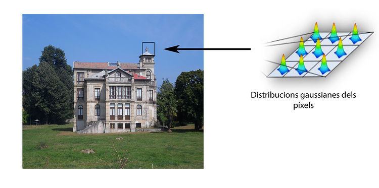
Background mixture models
Mixture of Gaussians method approaches by modelling each pixel as a mixture of Gaussians and uses an on-line approximation to update the model. In this technique, it is assumed that every pixel's intensity values in the video can be modeled using a Gaussian mixture model. A simple heuristic determines which intensities are most probably of the background. Then the pixels which do not match to these are called the foreground pixels. Foreground pixels are grouped using 2D connected component analysis.
At any time t, a particular pixel (
This history is modeled by a mixture of K Gaussian distributions:
where
First, each pixel is characterized by its intensity in RGB color space. Then probability of observing the current pixel is given by the following formula in the multidimensional case
Where the parameters are K is the number of distributions, ω is a weight associated to the ith Gaussian at time t with mean µ and standard deviation Σ .
Once the parameters initialization is made, a first foreground detection can be made then the parameters are updated. The first B Gaussian distribution which exceeds the threshold T is re-tained for a background distribution
The other distributions are considered to represent a foreground distribution. Then, when the new frame incomes at times
where k is a constant threshold equal to
Case 1: A match is found with one of the K Gaussians. For the matched component, the update is done as follows
Power and Schoonees [3] used the same algorithm to segment the foreground of the image
The essential approximation to
Case 2: No match is found with any of the
Once the parameter maintenance is made, foreground detection can be made and so on. An on-line K-means approximation is used to update the Gaussians. Numerous improvements of this original method developed by Stauffer and Grimson have been proposed and a complete survey can be found in Bouwmans et al. A standard method of adaptive backgrounding is averaging the images over time, creating a background approximation which is similar to the current static scene except where motion occur.
Surveys
Several surveys which concern categories or sub-categories of models can be found as follows:
Comparison
Several comparison/evaluation papers can be found in the literature:
Books
T. Bouwmans, F. Porikli, B. Horferlin, A. Vacavant, Handbook on "Background Modeling and Foreground Detection for Video Surveillance: Traditional and Recent Approaches, Implementations, Benchmarking and Evaluation", CRC Press, Taylor and Francis Group, June 2014. (For more information: http://www.crcpress.com/product/isbn/9781482205374)
T. Bouwmans, N. Aybat, and E. Zahzah. Handbook on Robust Low-Rank and Sparse Matrix Decomposition: Applications in Image and Video Processing, CRC Press, Taylor and Francis Group, May 2016. (more information: http://www.crcpress.com/product/isbn/9781498724623)