
 | ||
The Azimi Q models used Mathematical Q models to explain how the earth responds to seismic waves. Because these models satisfies the Krämers-Krönig relations they should be preferable to the Kolsky model in seismic inverse Q filtering.
Contents
Azimi's first model
Azimi's first model (1968), which he proposed together with Strick (1967) has the attenuation proportional to |w|1−γ and is:
The phase velocity is written:
Azimi's second model
Azimi's second model is defined by:
where a2 and a3 are constants. Now we can use the Krämers-Krönig dispersion relation and get a phase velocity:
Computations
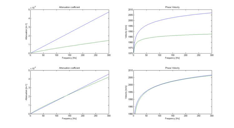
Studying the attenuation coefficient and phase velocity, and compare them with Kolskys Q model we have plotted the result on fig.1. The data for the models are taken from Ursin and Toverud.
Data for the Kolsky model (blue):
upper: cr=2000 m/s, Qr=100, wr=2π100
lower: cr=2000 m/s, Qr=100, wr=2π100
Data for Azimis first model (green):
upper: c∞=2000 m/s, a=2.5 x 10 −6, β=0.155
lower: c∞=2065 m/s, a=4.76 x 10 −6, β=0.1
Data for Azimis second model (green):
upper: c∞=2000 m/s, a=2.5 x 10 −6, a2=1.6 x 10 −3
lower: c∞=2018 m/s, a=2.86 x 10 −6, a2=1.51 x 10 −4