Autoencoder

Structure

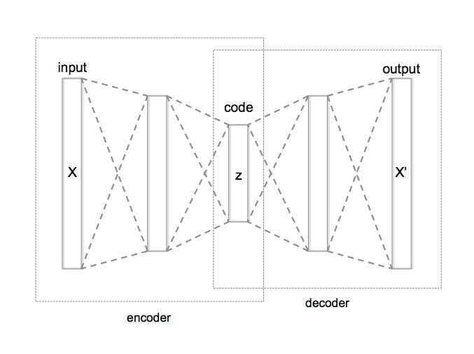
Architecturally, the simplest form of an autoencoder is a feedforward, non-recurrent neural network very similar to the multilayer perceptron (MLP) – having an input layer, an output layer and one or more hidden layers connecting them –, but with the output layer having the same number of nodes as the input layer, and with the purpose of reconstructing its own inputs (instead of predicting the target value Y given inputs X ). Therefore, autoencoders are unsupervised learning models.

An autoencoder always consists of two parts, the encoder and the decoder, which can be defined as transitions ϕ and ψ , such that:

ϕ : X → F ψ : F → X ϕ , ψ = arg ⁡ min ϕ , ψ ∥ X − ( ψ ∘ ϕ ) X ∥ 2

In the simplest case, where there is one hidden layer, an autoencoder takes the input x ∈ R d = X and maps it onto z ∈ R p = F :

z = σ 1 ( W x + b )

This is usually referred to as code or latent variables (latent representation). Here, σ 1 is an element-wise activation function such as a sigmoid function or a rectified linear unit. After that, z is mapped onto the reconstruction x ′ of the same shape as x :

x ′ = σ 2 ( W ′ z + b ′ )

Autoencoders are also trained to minimise reconstruction errors (such as squared errors):

L ( x , x ′ ) = ∥ x − x ′ ∥ 2 = ∥ x − σ 2 ( W ′ ( σ 1 ( W x + b ) ) + b ′ ) ∥ 2

If the feature space F has lower dimensionality than the input space X , then the feature vector ϕ ( x ) can be regarded as a compressed representation of the input x . If the hidden layers are larger than the input layer, an autoencoder can potentially learn the identity function and become useless. However, experimental results have shown that autoencoders might still learn useful features in these cases.

Variations

Various techniques exist to prevent autoencoders from learning the identity function and to improve their ability to capture important information and learn richer representations:

Denoising autoencoder

Denoising autoencoders take a partially corrupted input whilst training to recover the original undistorted input. This technique has been introduced with a specific approach to good representation. A good representation is one that can be obtained robustly from a corrupted input and that will be useful for recovering the corresponding clean input. This definition contains the following implicit assumptions:

The higher level representations are relatively stable and robust to the corruption of the input;

It is necessary to extract features that are useful for representation of the input distribution.

To train an autoencoder to denoise data, it is necessary to perform preliminary stochastic mapping x → x ~ in order to corrupt the data and use x ~ as input for a normal autoencoder, with the only exception being that the loss should be still computed for the initial input L ( x , x ~ ′ ) instead of L ( x ~ , x ~ ′ ) .

Sparse autoencoder

By imposing sparsity on the hidden units during training (whilst having a larger number of hidden units than inputs), an autoencoder can learn useful structures in the input data. This allows sparse representations of inputs. These are useful in pretraining for classification tasks.

Sparsity may be achieved by additional terms in the loss function during training (by comparing the probability distribution of the hidden unit activations with some low desired value), or by manually zeroing all but the few strongest hidden unit activations (referred to as a k-sparse autoencoder).

Variational autoencoder (VAE)

Variational autoencoder models inherit autoencoder architecture, but make strong assumptions concerning the distribution of latent variables. They use variational approach for latent representation learning, which results in an additional loss component and specific training algorithm called Stochastic Gradient Variational Bayes (SGVB). It assumes that the data is generated by a directed graphical model p ( x | z ) and that the encoder is learning an approximation q ϕ ( z | x ) to the posterior distribution p θ ( z | x ) where ϕ and θ denote the parameters of the encoder (recognition model) and decoder (generative model) respectively. The objective of the variational autoencoder in this case has the following form:

L ( ϕ , θ , x ) = D K L ( q ϕ ( z | x ) | | p θ ( z ) ) − E q ϕ ( z | x ) ( log ⁡ p θ ( x | z ) )

Here, D K L stands for the Kullback–Leibler divergence. The prior over the latent variables is set to be the centred isotropic multivariate Gaussian p θ ( z ) = N ( 0 , I ) .

Contractive autoencoder (CAE)

Contractive autoencoder adds an explicit regularizer in their objective function that forces the model to learn a function that is robust to slight variations of input values. This regularizer corresponds to the Frobenius norm of the Jacobian matrix of the encoder activations with respect to the input. The final objective function has the following form:

L ( x , x ′ ) + λ ∑ i | | ∇ x h i | | 2

Relationship with truncated singular value decomposition (TSVD)

If linear activations are used, or only a single sigmoid hidden layer, then the optimal solution to an autoencoder is strongly related to principal component analysis (PCA), as explained by Pierre Baldi in several papers.

Training

The training algorithm for an autoencoder can be summarized as

For each input x, Do a feed-forward pass to compute activations at all hidden layers, then at the output layer to obtain an output x ′ Measure the deviation of x ′ from the input x (typically using squared error), Backpropagate the error through the net and perform weight updates.

An autoencoder is often trained using one of the many variants of backpropagation (such as conjugate gradient method, steepest descent, etc.). Though these are often reasonably effective, there are fundamental problems with the use of backpropagation to train networks with many hidden layers. Once errors are backpropagated to the first few layers, they become minuscule and insignificant. This means that the network will almost always learn to reconstruct the average of all the training data. Though more advanced backpropagation methods (such as the conjugate gradient method) can solve this problem to a certain extent, they still result in a very slow learning process and poor solutions. This problem can be remedied by using initial weights that approximate the final solution. The process of finding these initial weights is often referred to as pretraining.

Geoffrey Hinton developed a pretraining technique for training many-layered "deep" autoencoders. This method involves treating each neighbouring set of two layers as a restricted Boltzmann machine so that the pretraining approximates a good solution, then using a backpropagation technique to fine-tune the results. This model takes the name of deep belief network.