Samiksha Jaiswal (Editor)

Approximate entropy

Updated on
Edit
Like
Comment
Share on FacebookTweet on TwitterShare on LinkedInShare on Reddit
Approximate entropy

In statistics, an approximate entropy (ApEn) is a technique used to quantify the amount of regularity and the unpredictability of fluctuations over time-series data.

Contents

For example, there are two series of data:

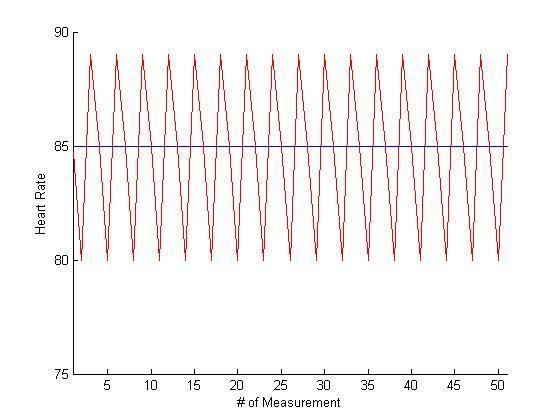
series 1: (10,20,10,20,10,20,10,20,10,20,10,20...), which alternates 10 and 20. series 2: (10,10,20,10,20,20,20,10,10,20,10,20,20...), which has either a value of 10 or 20, chosen randomly, each with probability 1/2.

Moment statistics, such as mean and variance, will not distinguish between these two series. Nor will rank order statistics distinguish between these series. Yet series 1 is "perfectly regular"; knowing one term has the value of 20 enables one to predict with certainty that the next term will have the value of 10. Series 2 is randomly valued; knowing one term has the value of 20 gives no insight into what value the next term will have.

Regularity was originally measured by exact regularity statistics, which has mainly centered on various entropy measures. However, accurate entropy calculation requires vast amounts of data, and the results will be greatly influenced by system noise, therefore it is not practical to apply these methods to experimental data. ApEn was developed by Steve M. Pincus to handle these limitations by modifying an exact regularity statistic, Kolmogorov–Sinai entropy. ApEn was initially developed to analyze medical data, such as heart rate, and later spread its applications in finance, psychology, and human factors engineering.

The algorithm

Step 1 : Form a time series of data   u ( 1 ) , u ( 2 ) , , u ( N ) . These are N raw data values from measurement equally spaced in time.

Step 2 : Fix   m , an integer, and   r , a positive real number. The value of   m represents the length of compared run of data, and   r specifies a filtering level.

Step 3 : Form a sequence of vectors x ( 1 ) , x ( 2 ) , , x ( N m + 1 ) , in R m , real   m -dimensional space defined by x ( i ) = [ u ( i ) , u ( i + 1 ) , , u ( i + m 1 ) ] .

Step 4 : Use the sequence x ( 1 ) , x ( 2 ) , , x ( N m + 1 ) to construct, for each   i , 1 i N m + 1

C i m ( r ) = ( number of  x ( j )  such that  d [ x ( i ) , x ( j ) ] r ) / ( N m + 1 )

in which   d [ x , x ] is defined as

d [ x , x ] = max a | u ( a ) u ( a ) |

The   u ( a ) are the m scalar components of x .   d represents the distance between the vectors x ( i ) and x ( j ) , given by the maximum difference in their respective scalar components. Note that j takes on all values, so the match provided when i = j will be counted (the subsequence is matched against itself).

Step 5 : Define

Φ m ( r ) = ( N m + 1 ) 1 i = 1 N m + 1 log ( C i m ( r ) ) ,

Step 6 : Define approximate entropy   ( A p E n ) as

  A p E n = Φ m ( r ) Φ m + 1 ( r ) .

where log is the natural logarithm, for   m and   r fixed as in Step 2.

Parameter selection: typically choose   m = 2 or   m = 3 , and   r depends greatly on the application.

An implementation on Physionet, which is based on Pincus use d [ x ( i ) , x ( j ) ] < r whereas the original article uses d [ x ( i ) , x ( j ) ] r in Step 4. While a concern for artificially constructed examples, it is usually not a concern in practice.

The interpretation

The presence of repetitive patterns of fluctuation in a time series renders it more predictable than a time series in which such patterns are absent. ApEn reflects the likelihood that similar patterns of observations will not be followed by additional similar observations. A time series containing many repetitive patterns has a relatively small ApEn; a less predictable process has a higher ApEn.

One example

Suppose   N = 51 , and the sequence consists of 51 samples of heart rate equally spaced in time:

  S N = { 85 , 80 , 89 , 85 , 80 , 89 , }

(i.e., the sequence is periodic with a period of 3). Let's choose   m = 2 and   r = 3 (the values of   m and   r can be varied without affecting the result).

Form a sequence of vectors:

x ( 1 ) = [ u ( 1 ) u ( 2 ) ] = [ 85 80 ] x ( 2 ) = [ u ( 2 ) u ( 3 ) ] = [ 80 89 ] x ( 3 ) = [ u ( 3 ) u ( 4 ) ] = [ 89 85 ] x ( 4 ) = [ u ( 4 ) u ( 5 ) ] = [ 85 80 ]

Distance is calculated as follows:

  d [ x ( 1 ) , x ( 1 ) ] = max a | u ( a ) u ( a ) | = 0 < r = 3

Note   | u ( 2 ) u ( 3 ) | > | u ( 1 ) u ( 2 ) | , so

  d [ x ( 1 ) , x ( 2 ) ] = max a | u ( a ) u ( a ) | = | u ( 2 ) u ( 3 ) | = 9 > r = 3

Similarly,

  d [ x ( 1 ) , x ( 3 ) ] = | u ( 2 ) u ( 4 ) | = 5 > r   d [ x ( 1 ) , x ( 4 ) ] = | u ( 1 ) u ( 4 ) | = | u ( 2 ) u ( 5 ) | = 0 < r

Therefore, x ( j ) s such that   d [ x ( 1 ) , x ( j ) ] r include x ( 1 ) , x ( 4 ) , x ( 7 ) , , x ( 49 ) , and the total number is 17.

  C 1 2 ( 3 ) = 17 50   C 2 2 ( 3 ) = 17 50   C 3 2 ( 3 ) = 16 50   C 4 2 ( 3 ) = 17 50  

Please note in Step 4, for x ( i ) ,   1 i N m + 1 . So the x ( j ) s such that   d [ x ( 3 ) , x ( j ) ] < r include x ( 3 ) , x ( 6 ) , x ( 9 ) , , x ( 48 ) , and the total number is 16.

Φ 2 ( 3 ) = ( 50 ) 1 i = 1 50 l o g ( C i 2 ( 3 ) ) 1.0982

Then we repeat the above steps for m=3. First form a sequence of vectors:

x ( 1 ) = [ u ( 1 ) u ( 2 ) u ( 3 ) ] = [ 85 80 89 ] x ( 2 ) = [ u ( 2 ) u ( 3 ) u ( 4 ) ] = [ 80 89 85 ] x ( 3 ) = [ u ( 3 ) u ( 4 ) u ( 5 ) ] = [ 89 85 80 ] x ( 4 ) = [ u ( 4 ) u ( 5 ) u ( 6 ) ] = [ 85 80 89 ]

By calculating distances between vector x ( i ) , x ( j ) , 1 i 49 , we find the vectors satisfying the filtering level have the following characteristic:

  d [ x ( i ) x ( i + 3 ) ] = 0 < r

Therefore,

  C 1 3 ( 3 ) = 17 49   C 2 3 ( 3 ) = 16 49   C 3 3 ( 3 ) = 16 49   C 4 3 ( 3 ) = 17 49   Φ 3 ( 3 ) = ( 49 ) 1 i = 1 49 l o g ( C i 3 ( 3 ) ) 1.0982

Finally,

A p E n = Φ 2 ( 3 ) Φ 3 ( 3 ) 0.000010997

The value is very small, so it implies the sequence is regular and predictable, which is consistent with the observation.

Advantages

The advantages of ApEn include:

  • Lower computational demand. ApEn can be designed to work for small data samples (n < 50 points) and can be applied in real time.
  • Less effect from noise. If data are noisy, the ApEn measure can be compared to the noise level in the data to determine what quality of true information may be present in the data.
  • Applications

    ApEn has been applied to classify EEG in psychiatric diseases, such as schizophrenia, epilepsy, and addiction.

    Limitations

    The ApEn algorithm counts each sequence as matching itself to avoid the occurrence of ln(0) in the calculations. This step might cause bias of ApEn and this bias causes ApEn to have two poor properties in practice:

    1. ApEn is heavily dependent on the record length and is uniformly lower than expected for short records.
    2. it lacks relative consistency. That is, if ApEn of one data set is higher than that of another, it should, but does not, remain higher for all conditions tested.

    References

    Approximate entropy Wikipedia