In electrical engineering, the alpha-beta ( α β γ ) transformation (also known as the Clarke transformation) is a mathematical transformation employed to simplify the analysis of three-phase circuits. Conceptually it is similar to the dq0 transformation. One very useful application of the α β γ transformation is the generation of the reference signal used for space vector modulation control of three-phase inverters.
The α β γ transform applied to three-phase currents, as used by Edith Clarke, is
i α β γ ( t ) = T i a b c ( t ) = 2 3 [ 1 − 1 2 − 1 2 0 3 2 − 3 2 1 2 1 2 1 2 ] [ i a ( t ) i b ( t ) i c ( t ) ] where i a b c ( t ) is a generic three-phase current sequence and i α β γ ( t ) is the corresponding current sequence given by the transformation T . The inverse transform is:
i a b c ( t ) = T − 1 i α β γ ( t ) = [ 1 0 1 − 1 2 3 2 1 − 1 2 − 3 2 1 ] [ i α ( t ) i β ( t ) i γ ( t ) ] . The above Clarke's transformation preserves the amplitude of the electrical variables which it is applied to. Indeed, consider a three-phase symmetric, direct, current sequence
i a ( t ) = 2 I cos θ ( t ) , i b ( t ) = 2 I cos ( θ ( t ) − 2 3 π ) , i c ( t ) = 2 I cos ( θ ( t ) + 2 3 π ) , where I is the RMS of i a ( t ) , i b ( t ) , i c ( t ) and θ ( t ) is the generic time-varying angle that can also be set to ω t without loss of generality. Then, by applying T to the current sequence, it results
i α = 2 I cos θ ( t ) , i β = 2 I sin θ ( t ) , i γ = 0 , where the last equation holds since we have considered balanced currents. As it is shown in the above, the amplitudes of the currents in the α β γ reference frame are the same of that in the natural reference frame.
The active and reactive powers computed in the Clark's domain with the transformation shown above are not the same of those computed in the standard reference frame. This happens because T is not unitary. In order to preserve the active and reactive powers one has, instead, to consider
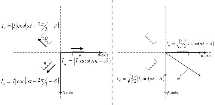
i α β γ ( t ) = T i a b c ( t ) = 2 3 [ 1 − 1 2 − 1 2 0 3 2 − 3 2 1 2 1 2 1 2 ] [ i a ( t ) i b ( t ) i c ( t ) ] , which is a unitary matrix and the inverse coincides with its transpose. In this case the amplitudes of the transformed currents are not the same of those in the standard reference frame, that is
i α = 3 I cos θ ( t ) , i β = 3 I sin θ ( t ) , i γ = 0. Finally, the inverse transformation in this case is
i a b c ( t ) = 2 3 [ 1 0 1 2 − 1 2 3 2 1 2 − 1 2 − 3 2 1 2 ] [ i α ( t ) i β ( t ) i γ ( t ) ] . Since in a balanced system i a ( t ) + i b ( t ) + i c ( t ) = 0 and thus i γ ( t ) = 0 one can also consider the simplified transform
i α β ( t ) = 2 3 [ 1 − 1 2 − 1 2 0 3 2 − 3 2 ] [ i a ( t ) i b ( t ) i c ( t ) ] which is simply the original Clarke's transformation with the 3rd equation thrown away, and
i a b c ( t ) = 3 2 [ 2 3 0 − 1 3 3 3 − 1 3 − 3 3 ] [ i α ( t ) i β ( t ) ] . The α β γ transformation can be thought of as the projection of the three phase quantities (voltages or currents) onto two stationary axes, the alpha axis and the beta axis.
The d q 0 transform is conceptually similar to the α β γ transform. Whereas the d q 0 transform is the projection of the phase quantities onto a rotating two-axis reference frame, the α β γ transform can be thought of as the projection of the phase quantities onto a stationary two-axis reference frame.