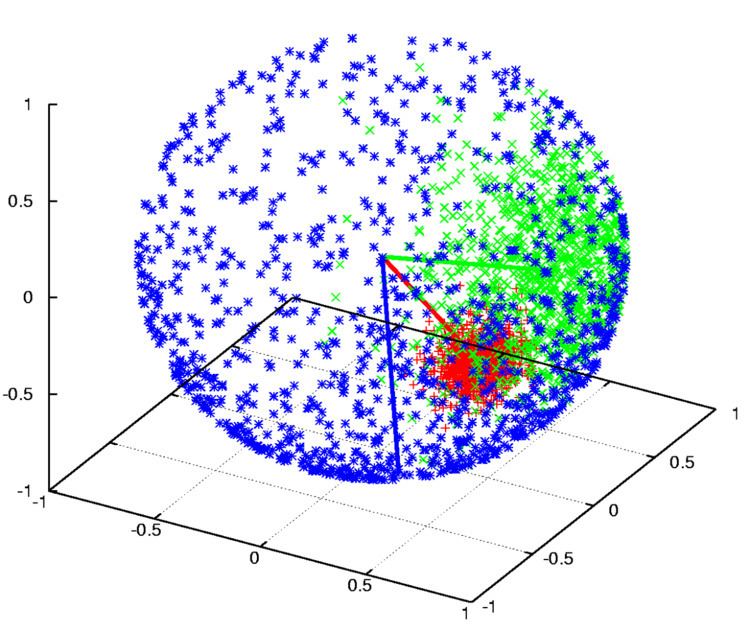
In directional statistics, the von Mises–Fisher distribution (named after Ronald Fisher and Richard von Mises), is a probability distribution on the
(
p
−
1
)
-dimensional sphere in
R
p
. If
p
=
2
the distribution reduces to the von Mises distribution on the circle.
The probability density function of the von Mises–Fisher distribution for the random p-dimensional unit vector
x
is given by:
f
p
(
x
;
μ
,
κ
)
=
C
p
(
κ
)
exp
(
κ
μ
T
x
)
where
κ
≥
0
,
∥
μ
∥
=
1
and the normalization constant
C
p
(
κ
)
is equal to
C
p
(
κ
)
=
κ
p
/
2
−
1
(
2
π
)
p
/
2
I
p
/
2
−
1
(
κ
)
.
where
I
v
denotes the modified Bessel function of the first kind at order
v
. If
p
=
3
, the normalization constant reduces to
C
3
(
κ
)
=
κ
4
π
sinh
κ
=
κ
2
π
(
e
κ
−
e
−
κ
)
.
The parameters
μ
and
κ
are called the mean direction and concentration parameter, respectively. The greater the value of
κ
, the higher the concentration of the distribution around the mean direction
μ
. The distribution is unimodal for
κ
>
0
, and is uniform on the sphere for
κ
=
0
.
The von Mises–Fisher distribution for
p
=
3
, also called the Fisher distribution, was first used to model the interaction of electric dipoles in an electric field (Mardia, 2000). Other applications are found in geology, bioinformatics, and text mining.
A series of N independent measurements
x
i
are drawn from a von Mises–Fisher distribution. Define
A
p
(
κ
)
=
I
p
/
2
(
κ
)
I
p
/
2
−
1
(
κ
)
.
Then (Sra, 2011) the maximum likelihood estimates of
μ
and
κ
are given by
μ
=
∑
i
N
x
i
∥
∑
i
N
x
i
∥
,
κ
=
A
p
−
1
(
R
¯
)
.
Thus
κ
is the solution to
A
p
(
κ
)
=
∥
∑
i
N
x
i
∥
N
=
R
¯
.
A simple approximation to
κ
is
κ
^
=
R
¯
(
p
−
R
¯
2
)
1
−
R
¯
2
,
but a more accurate measure can be obtained by iterating the Newton method a few times
κ
^
1
=
κ
^
−
A
p
(
κ
^
)
−
R
¯
1
−
A
p
(
κ
^
)
2
−
p
−
1
κ
^
A
p
(
κ
^
)
,
κ
^
2
=
κ
^
1
−
A
p
(
κ
^
1
)
−
R
¯
1
−
A
p
(
κ
^
1
)
2
−
p
−
1
κ
^
1
A
p
(
κ
^
1
)
.
For N ≥ 25, the estimated spherical standard error of the sample mean direction can be computed as
σ
^
=
(
d
N
R
¯
2
)
1
/
2
where
d
=
1
−
1
N
∑
i
N
(
μ
T
x
i
)
2
It's then possible to approximate a
100
(
1
−
α
)
%
confidence cone about
μ
with semi-vertical angle
q
=
arcsin
(
e
α
1
/
2
σ
^
)
,
where
e
α
=
−
ln
(
α
)
.
For example, for a 95% confidence cone,
α
=
0.05
,
e
α
=
−
ln
(
0.05
)
=
2.996
,
and thus
q
=
arcsin
(
1.731
σ
^
)
.

