Information Theory and Coding

Updated on Aug 21, 2018

Edit

Comment

http://www-ict.tf.uni-kiel.de/grafik/underwater_comm.jpg

Information theory is a branch of applied mathematics, electrical engineering, and computer science involving the quantification of information. Information theory was developed by Claude E. Shannon to find fundamental limits on signal processing operations such as compressing data and on reliably storing and communicating data. Since its inception it has broadened to find applications in many other areas, including statistical inference, natural language processing, cryptography, neurobiology, the evolution and function of molecular codes, model selection in ecology, thermal physics, quantum computing, plagiarism detection and other forms of data analysis.

A key measure of information is entropy, which is usually expressed by the average number of bits needed to store or communicate one symbol in a message. Entropy quantifies the uncertainty involved in predicting the value of a random variable. For example, specifying the outcome of a fair coin flip (two equally likely outcomes) provides less information (lower entropy) than specifying the outcome from a roll of a die (six equally likely outcomes).

Applications of fundamental topics of information theory include lossless data compression (e.g. ZIP files), lossy data compression (e.g. MP3s and JPEGs), and channel coding (e.g. for Digital Subscriber Line (DSL)). The field is at the intersection of mathematics, statistics, computer science, physics, neurobiology, and electrical engineering. Its impact has been crucial to the success of the Voyager missions to deep space, the invention of the compact disc, the feasibility of mobile phones, the development of the Internet, the study of linguistics and of human perception, the understanding of black holes, and numerous other fields. Important sub-fields of information theory are source coding, channel coding, algorithmic complexity theory, algorithmic information theory, information-theoretic security, and measures of information.

http://newsoffice.mit.edu/sites/mit.edu.newsoffice/files/images/2011/20110803175139-1_0.jpg

The main concepts of information theory can be grasped by considering the most widespread means of human communication: language. Two important aspects of a concise language are as follows: First, the most common words (e.g., "a", "the", "I") should be shorter than less common words (e.g., "roundabout", "generation", "mediocre"), so that sentences will not be too long. Such a tradeoff in word length is analogous to data compression and is the essential aspect of source coding. Second, if part of a sentence is unheard or misheard due to noise — e.g., a passing car — the listener should still be able to glean the meaning of the underlying message. Such robustness is as essential for an electronic communication system as it is for a language; properly building such robustness into communications is done by channel coding. Source coding and channel coding are the fundamental concerns of information theory.

Information theory is generally considered to have been founded in 1948 by Claude Shannon in his seminal work, "A Mathematical Theory of Communication". The central paradigm of classical information theory is the engineering problem of the transmission of information over a noisy channel. The most fundamental results of this theory are Shannons source coding theorem, which establishes that, on average, the number of bits needed to represent the result of an uncertain event is given by its entropy; and Shannons noisy-channel coding theorem, which states that reliable communication is possible over noisy channels provided that the rate of communication is below a certain threshold, called the channel capacity. The channel capacity can be approached in practice by using appropriate encoding and decoding systems.

Entropy & Types of Entropy
Entropy
The Entropy,

H

, of a discrete random variable

X

is a measure of the amount of uncertainty associated with the value of

X

Suppose one transmits 1000 bits (0s and 1s). If these bits are known ahead of transmission (to be a certain value with absolute probability), logic dictates that no information has been transmitted. If, however, each is equally and independently likely to be 0 or 1, 1000 bits (in the information theoretic sense) have been transmitted. Between these two extremes, information can be quantified as follows. If $\mathbb{X}$ is the set of all messages $\\{x_1, ..., x_n\\}$ that $X$ could be, and $p(x)$ is the probability of some $x \\in \\mathbb X$ , then the entropy, $H$ , of $X$ is defined:^[8]

H(X) = \\mathbb{E}_{X} [I(x)] = -\\sum_{x \\in \\mathbb{X}} p(x) \\log p(x).

(Here, $I(x)$ is the self-information, which is the entropy contribution of an individual message, and $\\mathbb{E}_{X}$ is the expected value.) An important property of entropy is that it is maximized when all the messages in the message space are equiprobable $p(x)=1/n$ ,—i.e., most unpredictable—in which case $H(X)=\\log n$ .

The special case of information entropy for a random variable with two outcomes is the binary entropy function, usually taken to the logarithmic base 2:

H_{\\mathrm{b}}(p) = - p \\log_2 p - (1-p)\\log_2 (1-p).\\,

Joint entropy
The Joint entropy of two discrete random variables

X

and

Y

is merely the entropy of their pairing:

(X, Y)

. This implies that if

X

and

Y

are independent, then their joint entropy is the sum of their individual entropies.

For example, if $(X,Y)$ represents the position of a chess piece — $X$ the row and $Y$ the column, then the joint entropy of the row of the piece and the column of the piece will be the entropy of the position of the piece.

H(X, Y) = \\mathbb{E}_{X,Y} [-\\log p(x,y)] = - \\sum_{x, y} p(x, y) \\log p(x, y) \\,

Despite similar notation, joint entropy should not be confused with cross entropy.

Conditional entropy (equivocation)
The Conditional entropy (equivocation) or Conditional uncertainty of

X

given random variable

Y

(also called the equivocation of

X

about

Y

) is the average conditional entropy over

Y

:^[9]

H(X|Y) = \\mathbb E_Y [H(X|y)] = -\\sum_{y \\in Y} p(y) \\sum_{x \\in X} p(x|y) \\log p(x|y) = -\\sum_{x,y} p(x,y) \\log \\frac{p(x,y)}{p(y)}.

Because entropy can be conditioned on a random variable or on that random variable being a certain value, care should be taken not to confuse these two definitions of conditional entropy, the former of which is in more common use. A basic property of this form of conditional entropy is that:

H(X|Y) = H(X,Y) - H(Y) .\\,

Mutual information (transinformation)
Mutual information measures the amount of information that can be obtained about one random variable by observing another. It is important in communication where it can be used to maximize the amount of information shared between sent and received signals. The mutual information of

X

relative to

Y

is given by:

I(X;Y) = \\mathbb{E}_{X,Y} [SI(x,y)] = \\sum_{x,y} p(x,y) \\log \\frac{p(x,y)}{p(x)\\, p(y)}

where $SI$ (Specific mutual Information) is the pointwise mutual information.

A basic property of the mutual information is that

I(X;Y) = H(X) - H(X|Y).\\,

That is, knowing Y, we can save an average of $I(X; Y)$ bits in encoding X compared to not knowing Y.

Mutual information is symmetric

I(X;Y) = I(Y;X) = H(X) + H(Y) - H(X,Y).\\,

Mutual information can be expressed as the average Kullback–Leibler divergence (information gain) between the posterior probability distribution of X given the value of Y and the prior distribution on X:

I(X;Y) = \\mathbb E_{p(y)} [D_{\\mathrm{KL}}( p(X|Y=y) \\| p(X) )].

In other words, this is a measure of how much, on the average, the probability distribution on X will change if we are given the value of Y. This is often recalculated as the divergence from the product of the marginal distributions to the actual joint distribution:

I(X; Y) = D_{\\mathrm{KL}}(p(X,Y) \\| p(X)p(Y)).

Mutual information is closely related to the log-likelihood ratio test in the context of contingency tables and the multinomial distribution and to Pearsons ?² test. mutual information can be considered a statistic for assessing independence between a pair of variables, and has a well-specified asymptotic distribution.

Kullback–Leibler divergence (information gain)
The Kullback–Leibler divergence (or information divergence, information gain, or relative entropy) is a way of comparing two distributions: a "true" probability distribution p(X), and an arbitrary probability distribution q(X). If we compress data in a manner that assumes q(X) is the distribution underlying some data, when, in reality, p(X) is the correct distribution, the Kullback–Leibler divergence is the number of average additional bits per datum necessary for compression. It is thus defined

D_{\\mathrm{KL}}(p(X) \\| q(X)) = \\sum_{x \\in X} -p(x) \\log {q(x)} \\, - \\, \\sum_{x \\in X} -p(x) \\log {p(x)} = \\sum_{x \\in X} p(x) \\log \\frac{p(x)}{q(x)}.

Although it is sometimes used as a distance metric, KL divergence is not a true metric since it is not symmetric and does not satisfy the triangle inequality (making it a semi-quasimetric).
Kullback–Leibler divergence of a prior from the truth

Another interpretation of KL divergence is this: suppose a number X is about to be drawn randomly from a discrete set with probability distribution p(x). If Alice knows the true distribution p(x), while Bob believes (has a prior) that the distribution is q(x), then Bob will be more surprised than Alice, on average, upon seeing the value of X. The KL divergence is the (objective) expected value of Bobs (subjective) surprisal minus Alices surprisal, measured in bits if the log is in base 2. In this way, the extent to which Bobs prior is "wrong" can be quantified in terms of how "unnecessarily surprised" its expected to make him.

Coding theory
Coding theory is one of the most important and direct applications of information theory. It can be subdivided into source coding theory and channel coding theory. Using a statistical description for data, information theory quantifies the number of bits needed to describe the data, which is the information entropy of the source.

Data compression (source coding): There are two formulations for the compression problem:
1. lossless data compression: the data must be reconstructed exactly;
2. lossy data compression: allocates bits needed to reconstruct the data, within a specified fidelity level measured by a distortion function. This subset of Information theory is called rate–distortion theory.

Error-correcting codes (channel coding): While data compression removes as much redundancy as possible, an error correcting code adds just the right kind of redundancy (i.e., error correction) needed to transmit the data efficiently and faithfully across a noisy channel.

http://content.answcdn.com/main/content/img/CDE/LOSSY.GIF

This division of coding theory into compression and transmission is justified by the information transmission theorems, or source–channel separation theorems that justify the use of bits as the universal currency for information in many contexts. However, these theorems only hold in the situation where one transmitting user wishes to communicate to one receiving user. In scenarios with more than one transmitter (the multiple-access channel), more than one receiver (the broadcast channel) or intermediary "helpers" (the relay channel), or more general networks, compression followed by transmission may no longer be optimal. Network information theory refers to these multi-agent communication models.

Source theory
Any process that generates successive messages can be considered a source of information. A memoryless source is one in which each message is an independent identically distributed random variable, whereas the properties of ergodicity and stationarity impose more general constraints. All such sources are stochastic. These terms are well studied in their own right outside information theory.

Channel capacity
Communications over a channel—such as an ethernet cable—is the primary motivation of information theory. As anyone whos ever used a telephone (mobile or landline) knows, however, such channels often fail to produce exact reconstruction of a signal; noise, periods of silence, and other forms of signal corruption often degrade quality. How much information can one hope to communicate over a noisy (or otherwise imperfect) channel?

Consider the communications process over a discrete channel. A simple model of the process is shown below:

Here X represents the space of messages transmitted, and Y the space of messages received during a unit time over our channel. Let $p(y|x)$ be the conditional probability distribution function of Y given X. We will consider $p(y|x)$ to be an inherent fixed property of our communications channel (representing the nature of the noise of our channel). Then the joint distribution of X and Y is completely determined by our channel and by our choice of $f(x)$ , the marginal distribution of messages we choose to send over the channel. Under these constraints, we would like to maximize the rate of information, or the signal, we can communicate over the channel. The appropriate measure for this is the mutual information, and this maximum mutual information is called the channel capacity and is given by:

C = \\max_{f} I(X;Y).\\!

This capacity has the following property related to communicating at information rate R (where R is usually bits per symbol). For any information rate R < C and coding error ? > 0, for large enough N, there exists a code of length N and rate ? R and a decoding algorithm, such that the maximal probability of block error is ? ?; that is, it is always possible to transmit with arbitrarily small block error. In addition, for any rate R > C, it is impossible to transmit with arbitrarily small block error.

Channel coding is concerned with finding such nearly optimal codes that can be used to transmit data over a noisy channel with a small coding error at a rate near the channel capacity.

Compression Algorithms
Huffman Coding
In computer science and information theory, a Huffman code is an optimal prefix code found using the algorithm developed by David A. Huffman while he was a Ph.D. student at MIT, and published in the 1952 paper "A Method for the Construction of Minimum-Redundancy Codes". The process of finding and/or using such a code is called Huffman coding, and is a common technique in entropy encoding, including in lossless data compression. The algorithms output can be viewed as a variable-length code table for encoding a source symbol (such as a character in a file). Huffmans algorithm derives this table based on the estimated probability or frequency (weight) of occurrence for each possible value of the source symbol. As in other entropy encoding methods, more common symbols are generally represented using fewer bits than less common symbols. Huffmans method can be efficiently implemented, finding a code in linear time to the number of input weights if these weights are sorted. However, although optimal among methods encoding symbols separately, Huffman coding is not always optimal among all compression methods.

Adaptive Huffman Compression
There are a few shortcomings to the straight Huffman compression. First of all, you need to send the Huffman tree at the beginning of the compressed file, or the decompressor will not be able to decode it. This can cause some overhead.

Also, Huffman compression looks at the statistics of the whole file, so that if a part of the code uses a character more heavily, it will not adjust during that section. Not to mention the fact that sometimes the whole file is not available to get the counts from (such as in live information).
The solution to all of these problems is to use an Adaptive method.

The Concept:
The basic concept behind an adaptive compression algorithm is very simple:

Initialize the model
Repeat for each character
{
Encode character
Update the model
}

Decompression works the same way. As long as both sides have the same initialize and update model algorithms, they will have the same information.

The problem is how to update the model. To make Huffman compression adaptive, we could just re-make the Huffman tree every time a character is sent, but that would cause an extermely slow algorithm. The trick is to only update the part of the tree that is affected.

The Algorithm:
The Huffman tree is initialized with a single node, known as the Not-Yet-Transmitted (NYT) or escape code. This code will be sent every time that a new character, which is not in the tree, is ecountered, followed by the ASCII encoding of the character. This allows for the decompressor to destinguish between a code and a new character. Also, the procedure creates a new node for the character and a new NYT from the old NYT node.

Whenever a character that is already in the tree is encountered, the code is sent and the weight is increased.

In order to for this algorithm to work, we need to add some additional information to the Huffman tree. In addition to each node having a weight, it will now also be assigned a unique node number. Also, all the nodes that have the same weight are said to be in the same block.

These node numbers will be assigned in such a way that:
1.   A node with a higher weight will have a higher node number.
2.   A parent node will always have a higher node number than its children.

This is known as the sibling property, and the update algorithm simply swaps nodes to make sure that this property is upheld. Obviously, the root node will have the highest node number because it has the highest weight.

Here is a flowchart of the update procedure,

http://www.cs.sfu.ca/CourseCentral/365/li/squeeze/update.gif

After a count is increased, the update procedure moves up the tree and inspects the ancestors of the node one at a time. It checks to make sure that the node have the highest node in its block, and if not, swaps it with the highest node number. It then increases the node weight and goes to the parent. It continues until it reaches the root node.
As you will see, this assures that the nodes with the highest weight are closer to the top and have shorter codes.

The Applet:
I realize that the update procedure is a little hard to understand, so I made this applet to demonstrate exactly what happens. The appplet creates and updates the tree while interactively sending over the characters. It also monitors the compression ratio of the string so far.

You can set the applet to Play-Pause or Continuous mode. In Play-Pause, a "Next Step" button pops up every time something is going to happen. You need to press this button to continue. In Continuous mode, the applet only pauses for 1 second in between steps.

LZW,RLE

Lempel–Ziv–Welch (LZW)
Lempel–Ziv–Welch (LZW) is a universal lossless data compression algorithm created by Abraham Lempel, Jacob Ziv, and Terry Welch. It was published by Welch in 1984 as an improved implementation of the LZ78 algorithm published by Lempel and Ziv in 1978. The algorithm is simple to implement, and has the potential for very high throughput in hardware implementations.[1] It was the algorithm of the widely used Unix file compression utility compress, and is used in the GIF image format.

Algorithm
The scenario described by Welchs 1984 paper encodes sequences of 8-bit data as fixed-length 12-bit codes. The codes from 0 to 255 represent 1-character sequences consisting of the corresponding 8-bit character, and the codes 256 through 4095 are created in a dictionary for sequences encountered in the data as it is encoded. At each stage in compression, input bytes are gathered into a sequence until the next character would make a sequence for which there is no code yet in the dictionary. The code for the sequence (without that character) is added to the output, and a new code (for the sequence with that character) is added to the dictionary.

The idea was quickly adapted to other situations. In an image based on a color table, for example, the natural character alphabet is the set of color table indexes, and in the 1980s, many images had small color tables (on the order of 16 colors). For such a reduced alphabet, the full 12-bit codes yielded poor compression unless the image was large, so the idea of a variable-width code was introduced: codes typically start one bit wider than the symbols being encoded, and as each code size is used up, the code width increases by 1 bit, up to some prescribed maximum (typically 12 bits).

Further refinements include reserving a code to indicate that the code table should be cleared (a "clear code", typically the first value immediately after the values for the individual alphabet characters), and a code to indicate the end of data (a "stop code", typically one greater than the clear code). The clear code allows the table to be reinitialized after it fills up, which lets the encoding adapt to changing patterns in the input data. Smart encoders can monitor the compression efficiency and clear the table whenever the existing table no longer matches the input well.

Since the codes are added in a manner determined by the data, the decoder mimics building the table as it sees the resulting codes. It is critical that the encoder and decoder agree on which variety of LZW is being used: the size of the alphabet, the maximum code width, whether variable-width encoding is being used, the initial code size, whether to use the clear and stop codes (and what values they have). Most formats that employ LZW build this information into the format specification or provide explicit fields for them in a compression header for the data.

http://www.j-a-b.net/web/graf/pics/gif_encoding

Run-length encoding (RLE)
Run-length encoding (RLE) is a very simple form of data compression in which runs of data (that is, sequences in which the same data value occurs in many consecutive data elements) are stored as a single data value and count, rather than as the original run. This is most useful on data that contains many such runs: for example, simple graphic images such as icons, line drawings, and animations. It is not useful with files that dont have many runs as it could greatly increase the file size.

RLE may also be used to refer to an early graphics file format supported by CompuServe for compressing black and white images, but was widely supplanted by their later Graphics Interchange Format. RLE also refers to a little-used image format in Windows 3.x, with the extension rle, which is a Run Length Encoded Bitmap, used to compress the Windows 3.x startup screen.

Typical applications of this encoding are when the source information comprises long substrings of the same character or binary digit.

Image Compression – GIF,JPEG

JPEG (Joint Photographic Experts Group)
JPEG is a standardised image compression mechanism. JPEG is designed for compressing either full-colour (24 bit) or grey-scale digital images of "natural" (real-world) scenes.

It works well on photographs, naturalistic artwork, and similar material; not so well on lettering, simple cartoons, or black-and-white line drawings (files come out very large). JPEG handles only still images, but there is a related standard called MPEG for motion pictures.
JPEG is "lossy", meaning that the image you get out of decompression isnt quite identical to what you originally put in. The algorithm achieves much of its compression by exploiting known limitation of the human eye, notably the fact that small colour details arent perceived as well as small details of light-and-dark. Thus, JPEG is intended for compressing images that will be looked at by humans.
A lot of people are scared off by the term "lossy compression". But when it comes to representing real-world scenes, no digital image format can retain all the information that impinges on your eyeball. By comparison with the real-world scene, JPEG loses far less information than GIF.

Quality v Compression
A useful property of JPEG is that the degree of lossiness can be varied by adjusting compression parameters. This means that the image maker can trade off file size against output image quality.

For good-quality, full-color source images, the default quality setting (Q 75) is very often the best choice. Try Q 75 first; if you see defects, then go up.

Except for experimental purposes, never go above about Q 95; using Q 100 will produce a file two or three times as large as Q 95, but of hardly any better quality. If you see a file made with Q 100, its a pretty sure sign that the maker didnt know what he/she was doing.
If you want a very small file (say for preview or indexing purposes) and are prepared to tolerate large defects, a Q setting in the range of 5 to 10 is about right. Q 2 or so may be amusing as "op art".

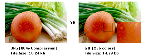
http://www.ntchosting.com/web_hosting_images/jpeg-vs-gif.jpg

GIF (Graphics Interchange Format)
The Graphics Interchange Format was developed in 1987 at the request of Compuserve, who needed a platform independent image format that was suitable for transfer across slow connections. It is a compressed (lossless) format (it uses the LZW compression) and compresses at a ratio of between 3:1 and 5:1

It is an 8 bit format which means the maximum number of colours supported by the format is 256.
There are two GIF standards, 87a and 89a (developed in 1987 and 1989 respectively). The 89a standard has additional features such as improved interlacing, the ability to define one colour to be transparent and the ability to store multiple images in one file to create a basic form of animation. Both Mosaic and Netscape will display 87a and 89a GIFs, but while both support transparency and interlacing, only Netscape supports animated GIFs.

Error Control Coding Techniques
In information theory and coding theory with applications in computer science and telecommunication, error detection and correction or error control are techniques that enable reliable delivery of digital data over unreliable communication channels. Many communication channels are subject to channel noise, and thus errors may be introduced during transmission from the source to a receiver. Error detection techniques allow detecting such errors, while error correction enables reconstruction of the original data.

types of code
1) Error Checking & Correcting Codes
2) Linear Block Codes
3) Cyclic Codes
4) BCH Codes
5) Convolution Codes

1) Error Checking & Correcting Codes
The general definitions of the terms are as follows:
1. Error detection is the detection of errors caused by noise or other impairments during transmission from the transmitter to the receiver.
2. Error correction is the detection of errors and reconstruction of the original, error-free data.

The general idea for achieving error detection and correction is to add some redundancy (i.e., some extra data) to a message, which receivers can use to check consistency of the delivered message, and to recover data determined to be corrupted. Error-detection and correction schemes can be either systematic or non-systematic: In a systematic scheme, the transmitter sends the original data, and attaches a fixed number of check bits (or parity data), which are derived from the data bits by some deterministic algorithm. If only error detection is required, a receiver can simply apply the same algorithm to the received data bits and compare its output with the received check bits; if the values do not match, an error has occurred at some point during the transmission. In a system that uses a non-systematic code, the original message is transformed into an encoded message that has at least as many bits as the original message.

Good error control performance requires the scheme to be selected based on the characteristics of the communication channel. Common channel models include memory-less models where errors occur randomly and with a certain probability, and dynamic models where errors occur primarily in bursts. Consequently, error-detecting and correcting codes can be generally distinguished between random-error-detecting/correcting and burst-error-detecting/correcting. Some codes can also be suitable for a mixture of random errors and burst errors.

If the channel capacity cannot be determined, or is highly variable, an error-detection scheme may be combined with a system for retransmissions of erroneous data. This is known as automatic repeat request (ARQ), and is most notably used in the Internet. An alternate approach for error control is hybrid automatic repeat request (HARQ), which is a combination of ARQ and error-correction coding.

2) Linear Block Codes
In coding theory, a linear code is an error-correcting code for which any linear combination of codewords is also a codeword. Linear codes are traditionally partitioned into block codes and convolutional codes, although turbo codes can be seen as a hybrid of these two types.Linear codes allow for more efficient encoding and decoding algorithms than other codes (cf. syndrome decoding).

Linear codes are used in forward error correction and are applied in methods for transmitting symbols (e.g., bits) on a communications channel so that, if errors occur in the communication, some errors can be corrected or detected by the recipient of a message block. The codewords in a linear block code are blocks of symbols which are encoded using more symbols than the original value to be sent. A linear code of length n transmits blocks containing n symbols. For example, the Hamming code is a linear binary code which represents 4-bit messages using 7-bit codewords. Two distinct codewords differ in at least three bits. As a consequence, up to two errors per codeword can be detected while a single error can be corrected. This code contains 24=16 codewords.

3) cyclic codes
In coding theory, a cyclic code is a block code, where the circular shifts of each codeword gives another word that belongs to the code. They are error-correcting codes that have algebraic properties that are convenient for efficient error detection and correction.
Let

\\mathcal{C}

be a linear code over a finite field

GF(q)

of block lenghth n.

\\mathcal{C}

is called a cyclic code if, for every codeword c=(c₁,...,c_n) from C, the word (c_n,c₁,...,c_n-1) in

GF(q)^n

obtained by a cyclic right shift of components is again a codeword. Because one cyclic right shift is equal to n ? 1 cyclic left shifts, a cyclic code may also be defined via cyclic left shifts. Therefore the linear code

\\mathcal{C}

is cyclic precisely when it is invariant under all cyclic shifts.

Cyclic Codes have some additional structural constraint on the codes. They are based on Galois fields and because of their structural properties they are very useful for error controls. Their structure is strongly related to Galois fields because of which the encoding and decoding algorithms for cyclic codes are computationally efficient.

4) BCH code
In coding theory, the BCH codes form a class of cyclic error-correcting codes that are constructed using finite fields. BCH codes were invented in 1959 by French mathematician Alexis Hocquenghem, and independently in 1960 by Raj Bose and D. K. Ray-Chaudhuri.The acronym BCH comprises the initials of these inventors names.

One of the key features of BCHodes is that during code design, there is a precise control over the number of symbol errors correctable by the code. In particular, it is possible to design binary BCH codes that can correct multiple bit errors. Another advantage of BCH codes is the ease with which they can be decoded, namely, via an algebraic method known as syndrome decoding. This simplifies the design of the decoder for these codes, using small low-power electronic hardware.

BCH codes are used in applications such as satellite communications, compact disc players, DVDs, disk drives, solid-state drives and two-dimensional bar codes.

Basic Number Theory
Modular Arithmetic
In mathematics, modular arithmetic is a system of arithmetic for integers, where numbers "wrap around" upon reaching a certain value—the modulus. The modern approach to modular arithmetic was developed by Carl Friedrich Gauss in his book Disquisitiones Arithmeticae, published in 1801.

http://www-history.mcs.st-and.ac.uk/~edmund/lnotes/img90.png

A familiar use of modular arithmetic is in the 12-hour clock, in which the day is divided into two 12-hour periods. If the time is 7:00 now, then 8 hours later it will be 3:00. Usual addition would suggest that the later time should be 7 + 8 = 15, but this is not the answer because clock time "wraps around" every 12 hours; in 12-hour time, there is no "15 oclock". Likewise, if the clock starts at 12:00 (noon) and 21 hours elapse, then the time will be 9:00 the next day, rather than 33:00. Since the hour number starts over after it reaches 12, this is arithmetic modulo 12. 12 is congruent not only to 12 itself, but also to 0, so the time called "12:00" could also be called "0:00", since 12 is congruent to 0 modulo 12.

This analogy is a little loose. The proper way to interpret this is that the group of integers modulo n act on the numbers of a clock, rather than the numbers on the clock being added together. Adding together two times on a clock is an example of a type error. However, it provides a useful way to understand the concept for the first time.

For a positive integer $n$ , two integers $a$ and $b$ are said to be congruent modulo $n$ , and written as

$a \\equiv b \\pmod n,\\,$
if their difference a ? b is an integer multiple of n (or n divides a ? b). The number n is called the modulus of the congruence, while integers congruent to a modulo n are creating a set called congruence class, residue class or simply residue of the integer a, modulo n. Congruence relation
Modular arithmetic can be handled mathematically by introducing a congruence relation on the integers that is compatible with the operations of the ring of integers: addition, subtraction, and multiplication. For a positive integer n, two integers a and b are said to be congruent modulo n, written:

$a \\equiv b \\pmod n,\\,$
if their difference a ? b is an integer multiple of n (or n divides a ? b). The number n is called the modulus of the congruence. For example,

38 \\equiv 14 \\pmod {12}\\,

because 38 ? 14 = 24, which is a multiple of 12.

The same rule holds for negative values:

\\begin{align} -8 &\\equiv 7 \\pmod 5\\\\ 2 &\\equiv -3 \\pmod 5\\\\ -3 &\\equiv -8 \\pmod 5\\, \\end{align}

Equivalently,

a \\equiv b \\pmod n\\,

can also be thought of as asserting that the remainders of the division of both a and b by n are the same. For instance:

38 \\equiv 14 \\pmod {12}\\,

because both 38 and 14 have the same remainder 2 when divided by 12. It is also the case that $38 - 14 = 24$ is an integer multiple of 12, which agrees with the prior definition of the congruence relation.

A remark on the notation: Because it is common to consider several congruence relations for different moduli at the same time, the modulus is incorporated in the notation. In spite of the ternary notation, the congruence relation for a given modulus is binary. This would have been clearer if the notation a ?_n b had been used, instead of the common

Chinese Remainder Theorem
The Chinese remainder theorem is a result about congruences in number theory and its generalizations in abstract algebra. It was first published in the 3rd to 5th centuries by Chinese mathematician Sun Tzu.

In its basic form, the Chinese remainder theorem will determine a number n that when divided by some given divisors leaves given remainders. For example, what is the lowest number n that when divided by 3 leaves a remainder of 2, when divided by 5 leaves a remainder of 3, and when divided by 7 leaves a remainder of 2?

Theorem statement
The original form of the theorem, contained in the 5th-century book Sunzis Mathematical Classic (????) by the Chinese mathematician Sun Tzu and later generalized with a complete solution called Dayanshu (???) in Qin Jiushaos 1247 Mathematical Treatise in Nine Sections (????, Shushu Jiuzhang), is a statement about simultaneous congruences.

Suppose n1, ..., nk are positive integers that are pairwise coprime. Then, for any given sequence of integers a1, ..., ak, there exists an integer x solving the following system of simultaneous congruences.

\\begin{cases} x \\equiv a_1 & \\pmod{n_1} \\\\ \\quad \\cdots \\\\ x \\equiv a_k &\\pmod{n_k} \\end{cases}

Furthermore, all solutions $x$ of this system are congruent modulo the product, $N = n 1 ... n k$ . Hence

x \\equiv y \\pmod{n_i}, \\quad 1 \\leq i \\leq k \\qquad \\Longleftrightarrow \\qquad x \\equiv y \\pmod{N}.

Sometimes, the simultaneous congruences can be solved even if the $n i$ are not pairwise coprime. A solution $x$ exists if and only if:

a_i \\equiv a_j \\pmod{\\gcd(n_i,n_j)} \\qquad \\text{for all }i\\text{ and }j

All solutions x are then congruent modulo the least common multiple of the ni.
Sun Tzus work contains neither a proof nor a full algorithm. What amounts to an algorithm for solving this problem was described by Aryabhata (6th century; see Kak 1986). Special cases of the Chinese remainder theorem were also known to Brahmagupta (7th century), and appear in Fibonaccis Liber Abaci (1202).

A modern restatement of the theorem in algebraic language is that for a positive integer with prime factorization

n = p_1^{r_1}\\cdots p_k^{r_k}

we have the isomorphism between a ring and the direct product of its prime power parts:

$\\mathbf{Z}/n\\mathbf{Z} \\cong \\mathbf{Z}/p_1^{r_1}\\mathbf{Z} \\times \\cdots \\times \\mathbf{Z}/p_k^{r_k}\\mathbf{Z}$
The theorem can also be restated in the language of combinatorics as the fact that the infinite arithmetic progressions of integers form a Helly family (Duchet 1995).

Fermat’s Little and Euler Theorem

Eulers theorem
In number theory, Eulers theorem (also known as the Fermat–Euler theorem or Eulers totient theorem) states that if n and a are coprime positive integers, then

a^{\\varphi (n)} \\equiv 1 \\pmod{n}

where ?(n) is Eulers totient function. (The notation is explained in the article Modular arithmetic.) In 1736, Euler published his proof of Fermats little theorem,[1] which Fermat had presented without proof. Subsequently, Euler presented other proofs of the theorem, culminating with "Eulers theorem" in his paper of 1763, in which he attempted to find the smallest exponent for which Fermats little theorem was always true.

The converse of Eulers theorem is also true: if the above congruence is true, then a and n must obviously be coprime.

The theorem is a generalization of Fermats little theorem, and is further generalized by Carmichaels theorem.

The theorem may be used to easily reduce large powers modulo n. For example, consider finding the ones place decimal digit of 7222, i.e. 7222 (mod 10). Note that 7 and 10 are coprime, and ?(10) = 4. So Eulers theorem yields 74 ? 1 (mod 10), and we get 7222 ? 74 × 55 + 2 ? (74)55 × 72 ? 155 × 72 ? 49 ? 9 (mod 10).

In general, when reducing a power of a modulo n (where a and n are coprime), one needs to work modulo ?(n) in the exponent of a:

if x ? y (mod ?(n)), then ax ? ay (mod n).

Eulers theorem also forms the basis of the RSA encryption system, where the net result of first encrypting a plaintext message, then later decrypting it, amounts to exponentiating a large input number by k?(n) + 1, for some positive integer k. Eulers theorem then guarantees that the decrypted output number is equal to the original input number, giving back the plaintext.

Fermats Little Theorem

Legendre and Jacobi Symbols
Jacobi symbol
The Jacobi symbol is a generalization of the Legendre symbol. Introduced by Jacobi in 1837, it is of theoretical interest in modular arithmetic and other branches of number theory, but its main use is in computational number theory, especially primality testing and integer factorization; these in turn are important in cryptography.

For any integer $a$ and any positive odd integer $n$ the Jacobi symbol is defined as the product of the legendre symbols corresponding to the prime factors of $n$ :

\\Bigg(\\frac{a}{n}\\Bigg) = \\left(\\frac{a}{p_1}\\right)^{\\alpha_1}\\left(\\frac{a}{p_2}\\right)^{\\alpha_2}\\cdots \\left(\\frac{a}{p_k}\\right)^{\\alpha_k}\\mbox{ where } n=p_1^{\\alpha_1}p_2^{\\alpha_2}\\cdots p_k^{\\alpha_k}

$\\left(\\tfrac{a}{p}\\right)$ represents the Legendre symbol, defined for all integers $a$ and all odd primes $p$ by

\\left(\\frac{a}{p}\\right) = \\begin{cases} \\;\\;\\,0\\mbox{ if } a \\equiv 0 \\pmod{p} \\\\+1\\mbox{ if }a \\not\\equiv 0\\pmod{p} \\mbox{ and for some integer }x, \\;a\\equiv x^2\\pmod{p} \\\\-1\\mbox{ if there is no such } x. \\end{cases}

Following the normal convention for the empty product, $\\left(\\tfrac{a}{1}\\right) = 1.$ The Legendre and Jacobi symbols are indistinguishable exactly when the lower argument is an odd prime, in which case they have the same value.

Calculating the Jacobi symbol
The above formulas lead to an efficient O((log a)(log b))[3] algorithm for calculating the Jacobi symbol, analogous to the Euclidean algorithm for finding the GCD of two numbers. (This should not be surprising in light of rule 3).

1. Reduce the "numerator" modulo the "denominator" using rule 2.
2. Extract any factors of 2 from the "numerator" using rule 4 and evaluate them using rule 8.
3. If the "numerator" is 1, rules 3 and 4 give a result of 1. If the "numerator" and "denominator" are not coprime, rule 3 gives a result of 0.
4. Otherwise, the "numerator" and "denominator" are now odd positive coprime integers, so we can flip the symbol using rule 6, then return to step 1.

Legendre symbol
In number theory, the Legendre symbol is a multiplicative function with values 1, ?1, 0 that is a quadratic character modulo a prime number p: its value on a (nonzero) quadratic residue mod p is 1 and on a non-quadratic residue (non-residue) is ?1. Its value on zero is 0.

The Legendre symbol was introduced by Adrien-Marie Legendre in 1798 in the course of his attempts at proving the law of quadratic reciprocity. Generalizations of the symbol include the Jacobi symbol and Dirichlet characters of higher order. The notational convenience of the Legendre symbol inspired introduction of several other "symbols" used in algebraic number theory, such as the Hilbert symbol and the Artin symbol.

Let p be an odd prime number. An integer a is a quadratic residue modulo p if it is congruent to a perfect square modulo p and is a quadratic nonresidue modulo p otherwise. The Legendre symbol is a function of a and p defined as follows:

\\left(\\frac{a}{p}\\right) = \\begin{cases} 1 & \\text{ if } a \\text{ is a quadratic residue modulo } p \\text{ and } a \\not\\equiv 0\\pmod{p} \\\\ -1 & \\text{ if } a \\text{ is a quadratic non-residue modulo } p \\\\ 0 & \\text{ if } a \\equiv 0 \\pmod{p}. \\end{cases}

Legendres original definition was by means of an explicit formula:

\\left(\\frac{a}{p}\\right) \\equiv a^{\\frac{p-1}{2}} \\pmod{p} \\quad \\text{ and } \\quad\\left(\\frac{a}{p}\\right) \\in \\{-1,0,1\\}.

By Eulers criterion, which had been discovered earlier and was known to Legendre, these two definitions are equivalent. Thus Legendres contribution lay in introducing a convenient notation that recorded quadratic residuosity of a mod p. For the sake of comparison, Gauss used the notation $a\\mathrm{R}p$ , $a\\mathrm{N}p$ according to whether a is a residue or a non-residue modulo p.

For typographical convenience, the Legendre symbol is sometimes written as (a|p) or (a/p). The sequence (a|p) for a equal to 0,1,2,... is periodic with period p and is sometimes called the Legendre sequence, with {0,1,?1} values occasionally replaced by {1,0,1} or {0,1,0}.